How filter pushdown works

Let’s imagine I have a database table — maybe a large collection of events, the sort of thing with a created_at timestamp and a few other columns. We’ll also imagine that I want fast, consistent queries as my data changes, so I’ve imported that table into Materialize.

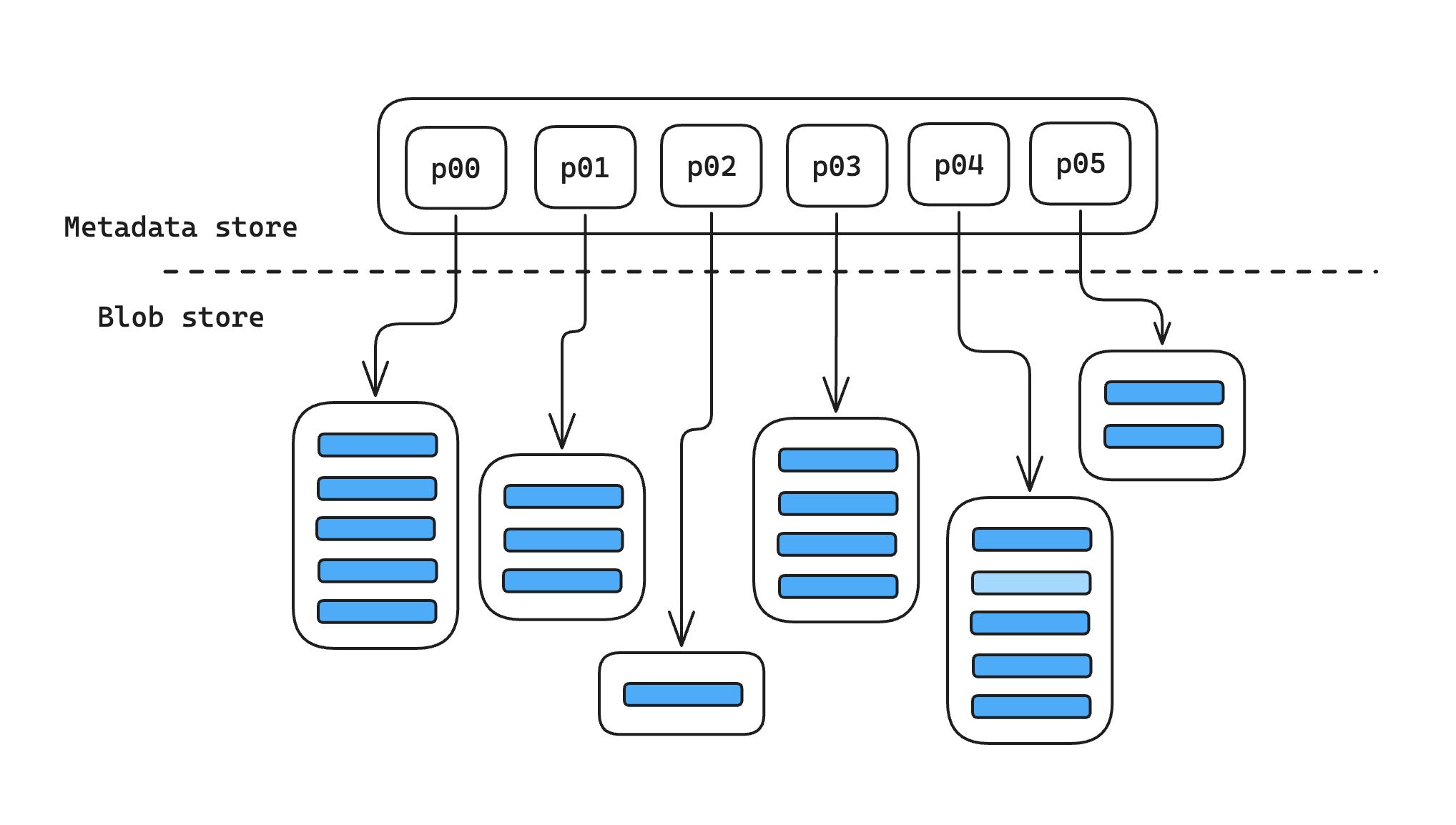
Materialize splits the data in a durable collection like this into multiple bounded-size parts, and stores each of those parts in an object store like S3. It stores the metadata separately, in a serializable store like CockroachDB or Postgres; this includes pointers to all the individual parts in the blob store, along with other metadata that Materialize needs to manage that collection as parts are added and removed over time.

Now suppose I’m trying to count up all the events that happened this year. I might write a query like:

SELECT count(*) from events
WHERE EXTRACT(YEAR FROM created_at) = 2025;

Materialize compiles this query down to a dataflow; in this precise case, you could think of it as a pipeline with roughly the following stages:

• Snapshot - examine the collection metadata and determine exactly which parts we’ll need to fetch from the blob store;
• Fetch - fetch and decode those parts, passing along the decoded row data;
• Filter - implement the WHERE clause, evaluating the filter expression and deciding whether to keep or discard each row;
• Reduce - do the actual count over all the rows that survive the filter.

Because of that filter, the reduce stage may only see a small fraction of the rows that are present in our collection. As it happens, it’s fairly common for all the rows that match a filter to be stored in just a small subset of the parts:

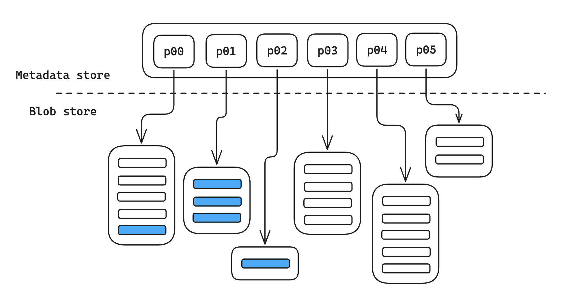
Perhaps I don’t have a ton of events yet in 2025, so there aren’t that many rows that match my filter; or perhaps I used partitioning to make sure that events at similar times were stored together; or perhaps I just got lucky. In any case, if the data I care about is clustered in just a few parts, that means there are a lot of parts that don’t include any data that I care about. Any time Materialize spends on those parts is wasted effort, since we’re going to immediately filter out all the data they contain. Ideally, we’d like some way to avoid fetching them at all.

Conveniently, Materialize has an optimization that handles exactly this — it can take the filter expression from the WHERE clause and apply it as part of that snapshot stage, using it to discard a bunch of parts that would otherwise need to be fetched. We call this operation filter pushdown, and it’s one of our most important low-level optimizations: on average it filters out about half the traffic to our object stores in our cloud deployment, and for queries that apply aggressive filters to well-partitioned datasets, it can cut latency by orders of magnitude. Many systems have a similar “predicate pushdown” or “pruning” optimization, but Materialize’s take on it is a bit unusual — using static analysis techniques to push down even complex filters within a running dataflow. In this post we’ll look at how filter pushdown works, why it works that way, and how it all shakes out in practice.

A toy example

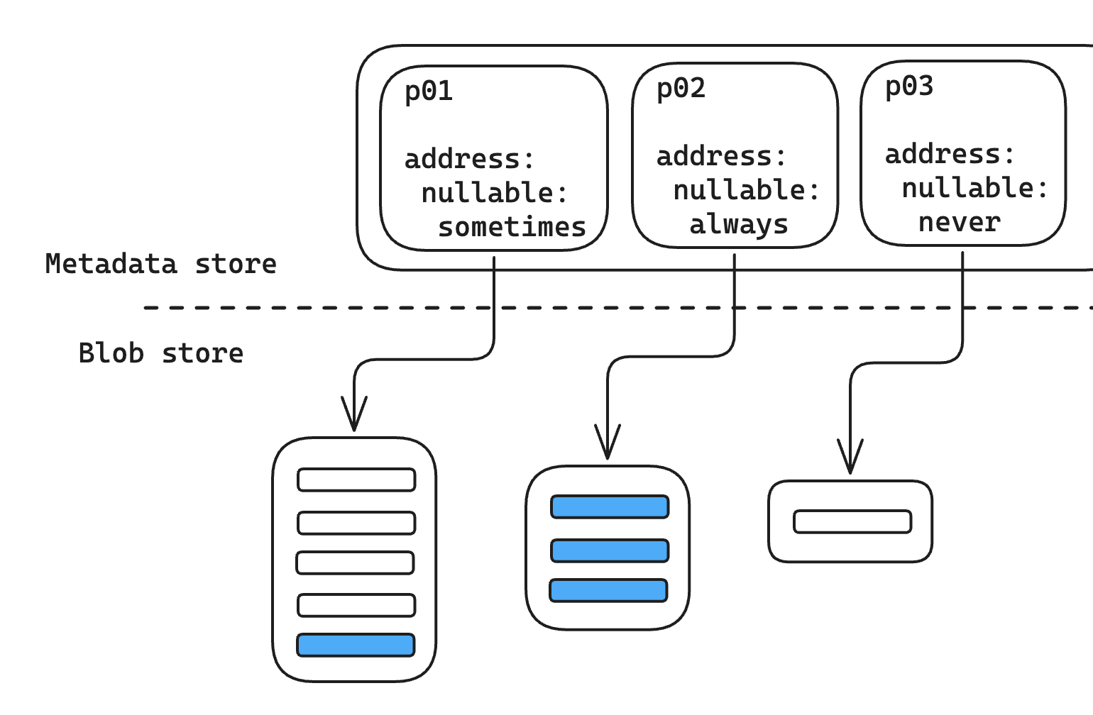
The full filter pushdown feature is a little complicated, so let’s start with a simpler case — filtering to rows where a particular column is null.

SELECT id FROM users WHERE address IS NULL;

This filter will discard any row with a non-null address. If we can figure out a part happens to consist entirely of rows with non-null addresses, we know none of those rows will contribute to our final result. One way to figure that out would be to fetch the part, decode it, then look to see whether that column contains any null values… but at that point we’ve already done all the work we’re trying to avoid!

Instead, we shift a little work to write time. Whenever we’re about to write a part, we look at every column in that part and decide whether it’s always null, sometimes null, or never null. This gives us a single nullable statistic for each column — and we write down all those statistics in the metadata, alongside our pointer to S3. Then, at read time, we can check those statistics. For our example query, we know that when we have nullable: never for our address column, the address IS NULL filter will filter out every row in that part, and skipping the fetch for that part won’t change our results.

nullable is an example of a “summary statistic” — a small bit of metadata that characterizes a chunk of data. Adding these statistics is a tradeoff: each statistic we add might let us filter more data and save a bunch of work at read time, but it also makes our writes slower and takes up precious space in our metadata store. For this sort of optimization to be worth it, we need to choose our statistics carefully and squeeze as much value out of them as we can.

Nullability analysis

Our simple nullable statistic can be used to push down very simple filters, but it turns out even this tiny statistic is good enough to help a little with some much more complex filters too. Consider a timestamp filter —

SELECT count(*) FROM events
WHERE EXTRACT(YEAR FROM created_at) = '2025';

This filter doesn’t explicitly mention null at all — but if created_at happens to be null and we interpret the filter, we’ll notice that:

• EXTRACT(YEAR FROM created_at) evaluates to null,
• null = '2025' also returns null,
• and when an entire filter expression evaluates to null the row is filtered out.

So: if our statistics for a particular part indicate that created_at is null for every row in that part, we know we’d end up filtering out all those rows, and we can skip fetching the part.

This sort of step-by-step reasoning makes our filter pushdown approach much more powerful. Instead of supporting just very simple null checks on nullable columns, we can use the same statistic to reason about arbitrarily complex expressions on arbitrary columns… as long as we know exactly when all of our functions and other subexpressions can return or propagate nulls.

That last bit isn’t trivial! While most SQL functions just return null just when they get a null as an argument, there are many that don’t — so for this sort of analysis to work, somebody needs to sit down and look at each of the functions that Materialize supports and check how they handle nulls. It turns out that “when can this function call return null” is important for all sorts of other optimizations too, so hardworking Materialize engineers had already done this work. Otherwise, doing this sort of analysis from scratch would have been fairly expensive.

Range analysis

Of course, if you have a filter like EXTRACT(YEAR FROM created_at) = '2025', you don’t just want to filter out parts where all the timestamps are null… you’d also love to filter out all the parts where all the rows have timestamps in 2024 or earlier. In general, many queries on many datasets filter by value, and it’d be very useful if we can push down filters deleted = false or blood_pressure > 140 as well.

To help with cases like this, we’re going to add a two new statistics: alongside our nullable statistic, we’ll track an upper and lower bound for data in the column. When we’re about to write a part, we’ll calculate those bounds for each column in the data and write them down in the metadata; when we’re about to read a part, we can use that range metadata to try and reason about the possible values that our function might return.

For example, if we know that the created_at for a particular row is between 2022-04-15 and 2024-06-01, we can conclude:

• EXTRACT(YEAR FROM created_at) would return 2022 for our lower bound and 2024 for our upper bound, so the actual value for our row must be somewhere in between;
• no number between 2022 and 2024 is equal to 2025, so ... = 2025 will definitely return false;
• and since our entire filter expression evaluates to false, the row gets filtered out.

This sort of range-based analysis has a shape very similar to our nullability analysis above, where we start from the statistics for individual columns and reason outward step-by-step, but in this case actually implementing each of those steps is trickier. In the worst case, we’d need a second implementation every SQL function we support — one that takes ranges as arguments and returns a range as a result — and the correct implementation for that function can be fairly subtle. (Even for a single function: EXTRACT(YEAR FROM ...) needs a totally different implementation from EXTRACT(MINUTE FROM ...), for example.)

We’re now also storing significantly more data: two new values per column in the dataset. This isn’t really an issue for simple types like timestamps and integers, but types like text can be arbitrarily large — and sometimes too large to inline into our part metadata. This gets handled in two ways:

• Some types like text can be truncated to fit. For example, if the minimum value in a column is 'OZARK', I know that all the values in that column must be >= 'OZ'.
• Some types can’t be truncated, and if we have a very large number of columns, even small per-column statistics can take up a lot of room in aggregate. In extreme cases like this, we may have to discard the statistics for certain columns entirely.

Abstract interpretation

Our first version of the filter pushdown optimization had these two part-level statistics, plus some read-time logic that looked for filters with certain patterns and did some ad-hoc reasoning. It worked pretty well for simple filters built on simple types, but Materialize’s users don’t only write simple filters… and many of the complex filters we saw in the wild would clearly benefit from filter pushdown if only we could make it slightly more clever. As we extended our code to handle more functions, more complex expressions, and more interesting types, that logic became increasingly tricky to maintain and debug. Small fixes that seemed safe, like truncation, would break implicit assumptions made far downstream. It was clear we needed more structure if we wanted to push this optimization any further.

Abstract interpretation is a general framework for this sort of program analysis, first developed in academic computer science but now used pretty widely in industry. For a theoretical explanation, Wikipedia is a good place to start; for a practical introduction, I like this blog post. But, to oversimplify — if we wanted to frame our problem in terms of abstract interpretation, we needed to come up with an abstract representation for two concrete things: values and functions. In return, abstract interpretation gave us a tool to use those basic pieces to reason about the behaviour of arbitrarily complex expressions… all with pretty strong guarantees about correctness.

Abstract values

Values like 3 or 'hello' or null are concrete values: they’re the sort of values that you might insert into a column in your database or receive as a result from a query. In abstract interpretation, our abstract values stand in for sets of concrete values like this. Sometimes these sets are pretty simple: for example, the literal 3 can only ever evaluate to a single value, so the set of all possible values for that literal is {3}. However, a column like bank_balance will have different values depending on the row — the abstract value for bank balance could have hundreds or millions of distinct values in the set, and the contents of that set will depend on the exact values of everybody’s bank account at any given time or in any given part.

Since these sets can be arbitrarily (or infinitely!) large, we can’t actually represent these abstract values in memory. Instead, we need to choose a representation for sets that’s more compact but still captures the distinctions we care about. In our case, our abstract values are defined by our summary statistics — our nullability statistic lets us pick out sets like “all non-null values”, and our range statistic describes sets like “all integers between 5 and 10 inclusive”. Abstract interpretation also has a couple rules for how we treat these abstract values, including:

• Our abstract values need to form a lattice. In practice, this requirement means that our abstract values behave like sets in important ways — for example, we can take the union or intersection of two abstract values, or represent the set of all possible values.
• Whenever we go from a set of concrete values to an abstract value, we need to be “conservative” and pick an abstract value that definitely includes every concrete value in the set. On the other hand, it’s fine if our abstract value includes some values that aren’t part of the set. This is a similar tradeoff to probabilistic data structures like a bloom filter: we may lose some precision, but we’ll never have a false negative.
• This is also exactly the right tradeoff for filter pushdown. It’s not a huge deal if we fetch a part and end up filtering all the rows, since the query will be a bit slower but still correct. On the other hand, failing to fetch a part that we were supposed to keep would be very bad!

We chose our abstract values based on the sort of data we wanted to deal with (typical SQL values) and the sort of expressions we wanted to interpret (typical SQL filter expressions). A C compiler might choose a totally different sort of abstract value representation to track the sort of distinctions that a C compiler cares about — whether particular bits are set or unset, for example. If the science of abstract interpretation is about making sure your abstract values don’t break the rules, the art is choosing an abstract value that’s right for your particular domain.

Abstract functions

In normal, “concrete” evaluation of a function, we pass specific concrete values as arguments and get a concrete result. For abstract interpretation we need a separate, “abstract” implementation of these functions that accepts abstract values and returns an abstract result.

In some cases, these functions are simpler to implement than the concrete function. When reasoning about nullability, many simple functions like sqrt can only return a null when passed a null as an argument, so their abstract implementation is pretty trivial. In other cases the abstract interpretation is more complex than the original — an implementation of sqrt for ranges involves taking the square root of both endpoints and needs special handling for zero and negative values.

Doing a special “abstract” reimplementation of all the functions Materialize supports could be a huge amount of work — possibly more work than it took to implement all those functions in the first place! For our particular application, though, we found a couple of tricks to make it manageable:

• We lean heavily on function annotations. Earlier, we mentioned that we could take advantage of existing nullability annotations to write a generic implementation instead of special-casing every function. As another example, a nice property of monotone functions is that you can figure out the min and max of the output range by just calling the function on the min and max of the input range, so we added a is_monotone annotation and use a shared generic implementation for all the functions that set it. It’s much easier to write one general implementation and then annotate a hundred functions than to write a hundred function-specific implementations from scratch!
• There are lots of functions and filters that just aren’t that interesting for filter pushdown. Take SELECT count(*) FROM events WHERE sha256(content) = '<digest>', for example: our nullability and range statistics just don’t tell us anything useful about which part might contain the row with a particular hash. For functions like this, we can just fall back to a default implementation that assumes a function might return anything at all.

Once you have abstract values for all the inputs for your expression, and abstract functions for all the functions in the expression, the actual interpretation process is pretty simple: we can just walk the AST and recursively evaluate each subexpression like we did in our examples above.

Putting it all together

That feels like enough theory for now — let’s walk through how this looks in practice for our actual production flow. For each part, Materialize will run through the following steps:

1. We translate the column stats from the part metadata to our abstract value type. This type includes our nullability and range stats, field-level stats for structured types like JSON, and additional metadata including the SQL type and whether an expression might error.
2. We run the actual abstract interpretation.
   • Literals get translated to the simplest possible abstract value that can represent them: a literal null becomes a nullable abstract value, and a literal number n becomes a non-nullable value with a range from n to n.
   • Column references get filled in with the abstract values we generated in step 1.
   • Function calls apply our abstract functions to our abstract values. Most functions bottom out at a generic implementation, which calls the concrete function with specific values and uses types and other metadata to infer its behaviour over all possible inputs, and falls back to a safe default if it can’t safely determine anything more specific. A few functions get custom implementations; for example, the try_parse_monotonic_iso8601_timestamp (which was carefully crafted to be pushed down even when normal timestamp parsing can’t be) gets equally special handling in the interpreter.
3. We check the result. Once abstract interpretation is complete, we end up with a new abstract value that represents the set of all possible results the filter expression might return. Finally, we ask: does that set contain true? (Or any errors? Mustn’t swallow errors.) If not, we’ve successfully proven that this expression will never return true for any row in our part, and we skip the fetch.

This analysis can be a little involved for complex filters — but it still ends up being much cheaper than fetching the data from the blob store, so it pays off if there’s even a small chance that we might get to skip the fetch.

Getting things right

Filter pushdown is a powerful optimization, but it’s also a risky one: if we ever decide to filter out a part that we should have kept, we risk returning the wrong results to the user. Like most features we ship, filter pushdown is tested in many ways at many levels of the database, from unit tests to large-scale integration testing… but there are a few ways we’ve given it special attention.

One of the nice things about the abstract interpretation formalism is that it gives us some pretty strong correctness properties. We’ve encoded these as a set of property tests that generate random datasets and random expressions, then runs both concrete and abstract interpretation over those datasets and checks that the results are consistent. These tests were very effective at finding bugs in development, both in the core interpreter logic and in the annotations on individual functions.

We also implemented a second, runtime safety feature we call “auditing”. When our abstract interpreter tells us that we don’t need to fetch a part, with some small probability we choose to fetch it anyways, then assert that all the contents really do get filtered out later. This was very useful as part of our feature-flagged rollout: by rolling out the feature incrementally across staging and production, we got a lot of additional confidence at a relatively small runtime overhead.

Building on filter pushdown

So: that’s a lot of work! What did we get for it?

It’s pretty easy to construct an example where filter pushdown works well. It tends to behave particularly well for temporal filters, which often select just a small percentage of recent data from a large dataset that’s partitioned nicely by time. In cases like this, filter pushdown can often winnow a multi-gigabyte dataset down to just a few dozen kilobytes, improving performance and cost by orders of magnitude.

Of course, for pretty much any optimization, it’s possible to tailor an example to make it look good. We’d really like to know how much the optimization helps in aggregate — whether it helps on real-world queries, and whether users run those queries often enough for it to be worth the trouble. One rough way to capture this is by comparing the number of bytes we filter out to the number of bytes we would have had to fetch if the optimization was turned off. Here’s that percentage, calculated across all clusters in one of our cloud regions:

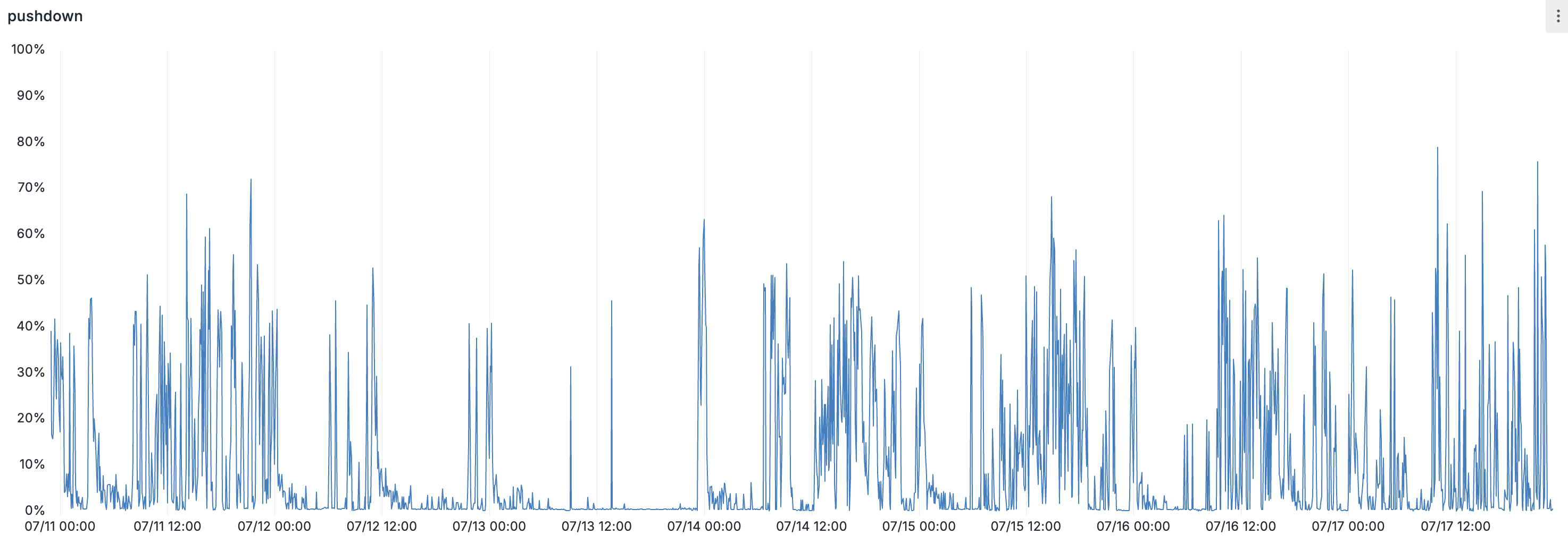
This metric is very spiky — filter pushdown tends to be most helpful when a large select query is being run or a new dataflow is being created, which is a little sporadic — but when it applies it often has a very large impact: there are hours where this optimization filters out more bytes than we fetch across the entire region. Of course, users don’t particularly care about our aggregate throughput — but every spike in this chart is a user hydrating a dataflow or running a query and having a much better experience than if they’d had to wait for Materialize to pull down all those bytes and then throw them away.

Are you interested in being one of the many Materialize users having good experiences and getting fast results? For more on when and how you can tailor your datasets and queries to get the most out of this optimization, see our documentation on partitioning and filter pushdown.