Understanding Differential Dataflow
January 11, 2021

I’ve been working at Materialize for almost a year now, and I have really enjoyed learning about and using Differential Dataflow (hereafter just Differential) in my day-to-day work.
In this post, I’ll introduce Differential and talk through implementing a few common programming problems like list intersection and everyone’s favorite, FizzBuzz, as dataflow programs. Finally, I’ll build a simple version of Conway’s Game of Life (hereafter just Life) in Differential.
My main goal is to describe how to write algorithms in Differential and give some intuition for when that’s a good idea. This post requires some knowledge of Rust to read the examples but otherwise assumes no prior background.
All the example code lives in a repository; you’ll just need to be able to build and run Rust programs to follow along!
What is Differential Dataflow?
Differential Dataflow is a framework that lets users define a computation using functional operations like map/join/reduce/etc. They send the computation inputs and modify the inputs, and sit back and watch the output and corresponding modifications to the outputs roll in. Differential will produce modifications to the outputs efficiently, without recomputing everything from scratch. Differential will even do this even when the computation has recursion.
Intersecting Lists in Differential Dataflow
Let’s start with a common interview problem: find the intersection (set of common elements) of two arrays of integers. This is probably one that most readers have seen before but still, let’s lay down a sketch of a fairly standard solution.
1 | |
2 | |
3 | |
4 | |
5 | |
6 | |
7 | |
8 | |
9 | |
10 | |
11 | |
12 | |
13 | |
14 | |
15 | |
16 | |
There’s some minor Rust specific things here but by and large this should feel familiar to everyone who has written code in an imperative language. We take two arrays of integers as input, transform them both into sets, and then go through the integers in one set to see if they’re also in the second. If so, we add them to our output. Pretty simple.
Let’s take a minute to appreciate two things: first, maintaining correct results over time while first and second changed arbitrarily would be hard, and second, we can’t reuse any of these pieces in Differential. We can’t convert arrays into hashsets because we only get collections, and we don’t have access to for loops because we don’t have access to control flow primitives.
Instead, we need to figure out a way to use dataflow operators. After digging around the docs for a bit, we can see that the semijoin operator looks very promising. semijoin takes two collections, one of type (Key, Value) and one of type (Key) and produces a collection of type (Key, Value) that contains all (k, v) pairs for keys with nonzero multiplicities in both collections. That’s not exactly the intersection we want but it’s awfully close.
Unfortunately, we aren’t fully out of the woods yet. It’s clear that we can use i32 as the key in both collections, but we don’t have any values. Thankfully, this is not a problem because we can use the unit type to simulate a value. We can use a map operator to turn a collection of type T into (T, ()).
Similarly, we can use another map to convert back from type (T, ()) to T. At this point, the output will be almost exactly what want, except that multiplicities in the output might be greater than one but we specifically want the intersection set. We can give the collection set semantics with the distinct operator. This implementation corresponds to the following dataflow graph.
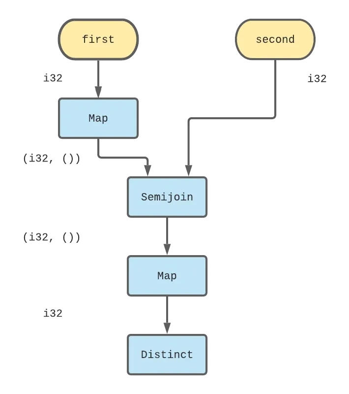
Here, edges represent collections, and blue rectangles represent dataflow operators. I’ve labelled first and second with yellow ovals to indicate that they are input collections that get data from external inputs, rather than from another operator’s output. I’ve also annotated each collection with its type to make the intent of the maps more clear. The Differential version of this graph looks like the following code:
1 | |
2 | |
3 | |
4 | |
5 | |
6 | |
Before we go any further, I want to call out three things.
First, this is one of many possible Differential solutions. For example, we could have used distinct on each of the inputs before we called semijoin. Alternatively, we could have used the join operator instead of the semijoin operator. All of these choices have various trade-offs that are unfortunately out of scope for this post but I want to highlight that it’s not as if
Differential is so strongly “declarative” that there’s only one canonical way to express a program. Second, I want to be really explicit about the relationship between the visual dataflow graph and the actual code. Every operator (blue rectangle) corresponds to one of the operator function calls in the code. Every incoming edge corresponds to one of the arguments to those functions, and every outgoing edge corresponds to one of the outputs of those functions.
Finally, and perhaps most importantly, we still don’t have the ability to send inputs to our dataflow operators and use all of this logic. We’ll need a bit more Differential and Timely (the underlying framework for distributed computation that Differential is built on) to get things going and the final result looks like:
1 | |
2 | |
3 | |
4 | |
5 | |
6 | |
7 | |
8 | |
9 | |
10 | |
11 | |
12 | |
13 | |
14 | |
15 | |
16 | |
17 | |
18 | |
19 | |
20 | |
21 | |
22 | |
23 | |
24 | |
25 | |
26 | |
We need to set up some Timely and Differential boilerplate here to get our computation going. We tell Timely to create a new dataflow graph with the dataflow method and can define our input collections with the new_collection method. new_collection gives us a “handle” which is basically like a pipe that we can use from elsewhere to send data into this collection, and a reference to the collection, that we can use within the closure to implement the actual graph (it’s the same logic as before). The only other novel bit in the closure is the inspect call which lets us print the contents of our collection to stdout.
The rest of the code outside of the closure deals with setting up an example. It’s sending integers to first and second at various logical times (based on when we advance_to) so that we can test out the logic. It’s not immediately obvious from the nested loop but first gets everything in [0, 19) (some of them repeated) and second gets everything in [5, 24) (again with repetitions). Therefore, the intersection set should be [5, 19) and indeed when I run this (you can see it too if you clone the repository) I see:
1 | |
2 | |
3 | |
4 | |
5 | |
6 | |
7 | |
8 | |
9 | |
10 | |
11 | |
12 | |
13 | |
14 | |
15 | |
16 | |
17 | |
18 | |
19 | |
20 | |
FizzBuzz in Differential Dataflow
I need to introduce one more operator before we can start working on Life, and like above, I’ll motivate it with a simple question: compute FizzBuzz for the numbers 1 - 100. An example solution is pretty simple.
1 | |
2 | |
3 | |
4 | |
5 | |
6 | |
7 | |
8 | |
9 | |
10 | |
11 | |
12 | |
This for-loop has a clear iterator 1..=100 that controls how many times the body of the loop executes. You could also choose to write it with a while loop like this:
1 | |
2 | |
3 | |
4 | |
5 | |
6 | |
Here, instead of directly specifying the number of iterations, I’ve specified a predicate that indicates when we should stop executing the loop. It’s a slightly different way to express the same idea. Differential has an operator for iteration called iterate but it doesn’t let you specify the iteration count, or a predicate to stop iterating. Instead, iterate repeatedly applies your logic (expressed as a dataflow fragment) to a collection until the output stops changing, aka reaches a fixed point. The process for writing dataflows like this feels less like writing a for loop, and more like writing an inductive proof. In that spirit I like to think of a partial result, and see what dataflow fragment would let us generate the next iterative result. More concretely, lets assume that we are storing our FizzBuzz data in a collection of type (i32, String) for simplicity and lets say that after four iterations, we have the following data:
1 | |
2 | |
3 | |
4 | |
We’d like now to take that collection as input and produce everything from above + (5, "Buzz") as output. Paradoxically, trying to be clever here and trying to find the maximum integer generated so far or something like that isn’t going to be very helpful. Instead, we’ll try the simpler strategy of having every single element to produce its “successor” (e.g. we’ll transform (2, "") into (3, "Fizz")) and then combine the set of successors with the existing set of inputs. As long as we are careful to only retain one copy of everything, the resulting output should be what we want. The dataflow graph for this single iteration logic looks like:
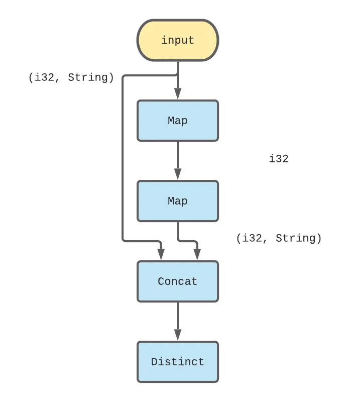
The corresponding code for that logic looks like the following.
1 | |
2 | |
3 | |
4 | |
5 | |
6 | |
7 | |
8 | |
9 | |
10 | |
11 | |
12 | |
13 | |
14 | |
The second map ends up being exactly the same for-loop as in the imperative version! From here, we just need to encode logic that will make the collection stop at 100. Remember, we can’t control how many times the dataflow computation will execute but we can control what we emit as output. In this case, we can use a filter operator to restrict our FizzBuzz output to [1, 100]. We can now take our logic for handling a single iteration of FizzBuzz and use it as the logic for iterate. This is our final dataflow graph for FizzBuzz:
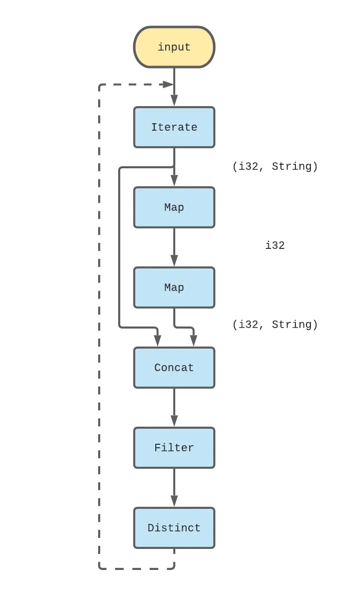
The final Differential code for FizzBuzz should look familiar at this point.
1 | |
2 | |
3 | |
4 | |
5 | |
6 | |
7 | |
8 | |
9 | |
10 | |
11 | |
12 | |
13 | |
14 | |
15 | |
16 | |
17 | |
18 | |
19 | |
20 | |
21 | |
22 | |
23 | |
24 | |
25 | |
26 | |
27 | |
28 | |
Life in Differential Dataflow
Let’s briefly touch on the rules. We have a (infinite) grid of square cells. All cells have 8 adjacent neighbors and all the cells are either “dead” or “live”, and the game evolves in discrete rounds as follows:
- Any live cell with two or three live neighbors stays live in the next round. (moral of the story: you need to have friends but not too many)
- Any dead cell with three live neighbors becomes live in the next round (this is how babies are made)
- All other live cells die in the next round. All other dead cells stay dead in the next round. (some cells die of natural causes, some get killed by their neighbors; no zombies)
Let’s start by imagining how we might do this in an imperative language. We could, for example, use an array to store the cells, and use a doubly nested for-loop to iterate through cells and evolve their state over rounds. I won’t bother writing down a full Rust implementation because clearly, this won’t give us a lot of insight into how to express it in terms of a dataflow graph.
Instead, let’s make some concrete decisions about how we want to represent this problem as collections and see if we can sketch out what we would need to do to make things work. I propose that we represent cells using pairs of integers (x, y) indicating their coordinates in the grid and furthermore, that we keep a collection of cells that are “live” at a round, and use iterate to evolve that collection over rounds. Unlike FizzBuzz, Life isn’t guaranteed to terminate. For now, let’s ignore that and revisit it later.
We’re in a position pretty similar to the one we were in earlier. We want to write a dataflow graph that can take in a set of pairs as input, and produce a new set of pairs as output. Unlike FizzBuzz, there isn’t a natural mapping from each input element to an output element. Instead, outputs depend on the numbers of live neighbors each cell has.
In an imperative setting, we might write code that asks “how many of my neighbors were live?” for each cell in the grid. In Differential, we’ll have an easier time if we let each live cell announce “these are my neighbors!” and then count how many live cells each announced neighbor was adjacent to.
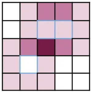
It’s hard to describe the idea fully in prose so let’s go through a visual example. Imagine that this is the state of our grid at some round, and the cells shaded in blue are live, and the rest are dead.
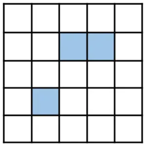
We can visualize the potentially live cells in the next round as follows. Only filled in cells below had at least one live neighbor this round, and so they are the only ones who might be live in the next round. The cells shaded in light pink had exactly one live neighbor, the cells shaded in pink had two live neighbors, and the one cell in the very center that’s shaded in dark magenta has three live neighbors.
That’s the only cell that will be live in the next round. The cells with blue borders represent the cells that were themselves live in the preceding round but unfortunately none of them had enough live neighbors to make it through to the next. We want to write a dataflow fragment that starts with the previously live cells (the blue cells from above), and gives potentially live cells (shaded cells below), before filtering down to only live ones in the next round.
First, we have to get each live cell to propose all of its neighbors. Fortunately, we can do that with a little bit of arithmetic.
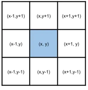
We can use the flat_map operator to do this arithmetic and generate 8 neighbors from each live cell, and then we can count the number of times each neighbor was emitted (by a formerly live cell) to end up with a collection of potentially eligible cells and the number of live neighbors each of them had. I’ve added some English annotations on the right to go along with the type signatures of each collection on the left.
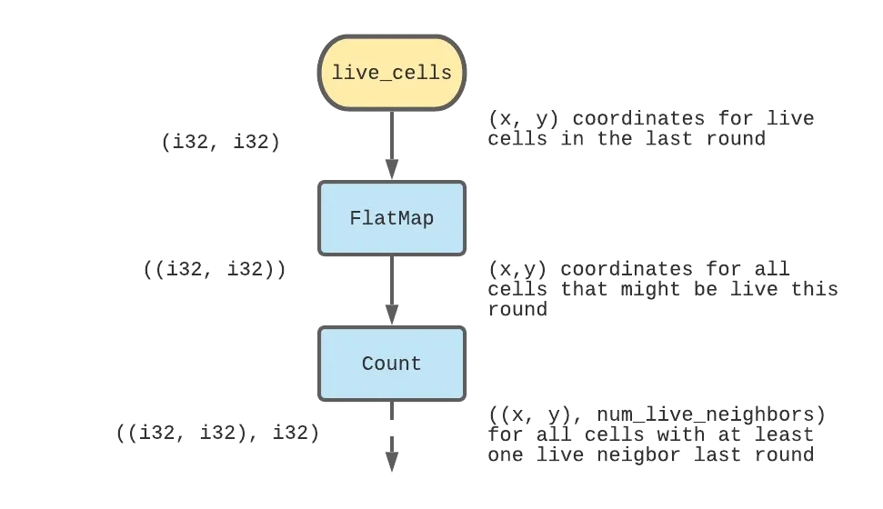
The code for this part is:
1 | |
2 | |
3 | |
4 | |
5 | |
6 | |
7 | |
8 | |
9 | |
10 | |
11 | |
12 | |
13 | |
14 | |
15 | |
16 | |
Next, we need to figure out a way now to apply the evolution rules 1 - 3 above to this collection of maybe_live_cells. As written, those rules require us to know “was this cell live in the previous round” which we don’t currently have access to. But if we transpose rules 1 and 2 a little bit, we can rewrite them as:
- all cells that have 3 live neighbors are live in the next round.
- all cells that have 2 live neighbors and are currently live stay live in the next round.
This now lets us take action based on the data we have. We can filter out the set of cells with 3 live neighbors; all of these cells will be live in the next round. We can also filter out the set of cells with 2 live neighbors, and now semijoin them against the live_cells from before to figure out which of these were previously live. Finally, we can concat the two result collections together, and that’s the set of live cells in the next round! As with FizzBuzz, this logic describes a single iteration of Life, and we can place the whole thing inside of an iterate loop and that’s pretty much the full implementation.
Let’s take a step back and look at the dataflow graph I’ve only verbally described so far.
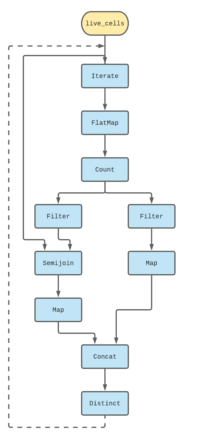
The code for this snippet, which does the logic for Life, follows pretty closely:
1 | |
2 | |
3 | |
4 | |
5 | |
6 | |
7 | |
8 | |
9 | |
10 | |
11 | |
12 | |
13 | |
14 | |
15 | |
16 | |
17 | |
18 | |
19 | |
20 | |
21 | |
22 | |
23 | |
24 | |
25 | |
26 | |
27 | |
28 | |
29 | |
30 | |
31 | |
32 | |
And that's pretty much it! We can run this (the rest of the code in src/main.rs seeds the computation with a list of starting live cells so that Life converges in a few rounds).
1 | |
2 | |
3 | |
4 | |
5 | |
6 | |
7 | |
8 | |
9 | |
10 | |
11 | |
12 | |
13 | |
It’s not the most thrilling graphics :). You can edit the list of starting cells to see more complex and infinitely evolving grids with fun things like gliders or other more exotic automata. While this is technically a working Game of Life implementation, it’s not very useful at the moment because we can’t ask it to evolve say, the next 20 iterations.
It’s all or nothing and it won’t stop until the game state converges to a fixed point which might never happen. We’ll fix all of these things, and compare the Differential version’s performance against a more standard implementation in the next post. Also, we’ll show off some pretty mind-bending time travel-esque things Differential lets you do with partially ordered times that would be pretty hard to do by hand.
If you thought this post was cool and want to learn more about Differential, you should check out the mdbook. If you want to see an example of Differential being used in the real world you should check out the Materialize source code!
Thanks Andi, Eli, Frank, Justin, Matt and Paul for reading earlier versions of this post and providing valuable feedback.
