Maintaining Joins using Few Resources

Today's post is on a topic that a lot of folks have asked for, once they dive a bit into Materialize.
One of our join implementation strategies uses a surprisingly small amount of additional memory: none. "None" is a surprising amount of memory because streaming joins normally need to maintain their inputs indexed in memory. Clearly there is a catch!
In a sense, there is. For the efficient plan to apply, you must have pre-built several indexes over the involved data. Materialize can share pre-built indexes between queries, like you might expect from a relational database, but unlike most stream processors. Once those indexes are in place, each additional query requires no additional memory for its joins. So there is a fixed up-front cost for each of your relations, but then no per-query cost as you join those relations multiple ways.
There is a lot of interesting stuff to learn, so let's get started! By the end of the post, I hope you'll be able to put together queries that use fewer resources, and understand some of the mystery behind it!
Materialize
Materialize is a system that allows you to express SQL queries over continually changing sources of data. These changes are first class citizens in Materialize, rather than just "whatever happens to the data". In particular, Materialize manipulates streams of "updates": triples (data, time, diff) where:
datais the where of the update: what record changed.timeis the when of the update: at what moment should it take effect.diffis the what of the update: how many copies ofdatado we add or remove.
These streams of updates describe a continually changing collection, whose contents at any time t are determined by adding up the updates whose time is less or equal to t. Specifically, the collection contains as many copies of data as the accumulation of diff in those updates. That number might be zero, in which case data is absent from the collection. It probably shouldn't be a negative number, which would suggest that something has gone wrong. It could be a large positive number which just means that there are multiple copies of data.
With these streams of updates, Materialize builds dataflows of operators that transform update streams for input collections into update streams for output collections. Dataflows are built out of operators, and larger computations still can be formed by composing dataflows. Ultimately, Materialize maintains multiple dataflows of updates that correctly compute and then consistently maintain the updates to arbitrary SQL views.
To do all of this, we at Materialize need to be able to build dataflow fragments that implement the various parts of SQL views. We are going to look at the specific case of doing that for the workhorse: a multiway relational join.
Relational Joins
In SQL a relational join of two collections is the new collection that contains all pairs of records one from each collection. The columns of the paired records are usually concatenated, to form a collection with all of the columns present in each input. A multiway relational join is this, but for any number of input collections, not just two.
Folks usually don't want all pairs, and so joins often come with constraints, which are predicates that restrict down the final set of records. Rather than produce all pairs (or triple, or quadruplets, etc), implementations will usually lean hard on the constraints to restrict their attention to the results that could possibly emerge in the output.
For example, consider this actual join fragment from TPCH query 3:
1 | |
2 | |
3 | |
4 | |
5 | |
6 | |
7 | |
8 | |
9 | |
10 | |
11 | |
12 | |
This query considers all triplets of data from customer, orders, and lineitem. However, the query also narrows this down to records that satisfy other constraints. Some of these constraints are on columns from just one input (e.g. c_mktsegment = 'BUILDING'). Some of these constraints relate columns from different inputs (e.g. AND c_custkey = o_custkey).
While the constraints on single inputs reduce the data, it is the constraints on columns from different inputs that really narrows our focus. Rather than match all records from customer and orders, we know that matches will have the same custkey column. We can group each of these collections by their custkey column, consider pairs that match, and never consider pairs that do not match. We've reduced down the amount of work from certainly quadratic (|customer| x |orders|) to something linear in the input (to read and group the input by these key columns) and the output (to enumerate each of the outputs). This improvement can be substantial, and can be even more substantial as we add more relations.
As we add more relations, we would like to do the same trick. The lineitem relation doesn't have a custkey column, and even if it did it isn't used in a constraint. Instead, we need to think about taking the output of the binary join above, and repeating the process with the orderkey column. Nothing wrong with doing that, and we end up only considering the pairs that might match on orderkey, which is again great news.
There are other ways we could have done the same thing. We could have started with lineitem and orders, and then added in customer. We could have started with lineitem and customer, and then added in orders. The first of these is a fine idea, but the second one has some flaws. The lineitem and customer relations don't share a constraint, so what could we use? We'd end up taking all pairs again, which probably doesn't end up better than the other approaches (it can in some cases, but it isn't the common case).
All of this is to say: when faced with a multiway relational join, we have some options in front of us for how to perform it. We haven't even enumerated all of the options, and they are going to become even more varied as we head to streaming updates rather than static data.
Relational Joins on Update Streams
The problem Materialize faces is maintaining multiway relational joins over inputs presented as streams of updates. Specifically, we need to build .. something .. that can translate input streams of updates to an output stream of updates. That output stream of updates must have the property that at all times t it accumulates to the collection that is the correct answer to the multiway relational join applied to the accumulation of each of the inputs at time t.
One (not great) approach is to fully re-form each of the inputs at each time t and repeat the query to see the output, and then subtract out whatever was previously produced. If there are new records they will be produced as + diffs, and if records are now missing they will be produced as - diffs. Unfortunately, this approach does an amount of work proportional to the total size of the data, even if not very much has changed. We'd love to take advantage of the fact that we are pointed at the input changes, and perhaps leap more-or-less directly from them to the output changes.
In fact, many relational databases do this already, although not in the streaming context.
Let's consider that three-way join from above, and ask "what if someone gave us a table d_customer that contained some additions to customer?" Let's say we've already computed the join on the prior customer relation and just want to know what additions there will be in the output. If we use the distributive property, we can conclude that
1 | |
2 | |
3 | |
If you believe this math, then you can see that we can go from the prior value of the join (the first line) to the new value of the join (the last line) by adding in a correction term that uses d_customer in place of customer (the second line). The SQL query that figures this out the correction for us is:
1 | |
2 | |
3 | |
4 | |
5 | |
6 | |
7 | |
8 | |
9 | |
10 | |
11 | |
12 | |
Superficially, this looks pretty identical to our original query, but with d_customer in place of customer. This is the case, and it will repeat itself for each of the other inputs. You might want a moment to convince yourselves that the WHERE constraints at the end don't change the correctness. These constraints also distribute over +, so it is fine to do them on parts of an update that we then add together.
However, HOWEVER! These filters play a really interesting role now.
First, let's agree that you could have done the same thing up above with a d_orders or with a d_lineitem. They each produce a query that would describe additions to the output from additions to the specific input. The only differences between the queries is which of the base relations we've substituted with a d_ relation.
The "really interesting" thing (to me, at least) is that these three queries, starting from different d_ relations, can have very different query plans. Remember how up above the WHERE constraints led us to consider different ways to evaluate a query, where we started with one pair of relations, and then joined in the third? We are going to do that again, but we can make different choices for each of the three update queries.
Generally, the d_ update relations are smaller than their base relations. It isn't always the case, but it is the main premise of streaming updates around instead of recomputing things from scratch. Given that, it makes a lot of sense to start each of the three update queries with its respective d_ relation. Based on the constraints, it makes a lot of sense to follow these relations with relations they share a constraint with.
Parenthesizing to show off the intended order of joins, and based on the constraints we have, we are interested in performing the joins as:
1 | |
2 | |
3 | |
The second line could have gone either way, perhaps starting with d_orders x lineitem instead. However, the first and last line are different plans, and they are each the right way to respond to changes to customer and lineitem respectively.
Here is a picture of the three queries, written as dataflows.
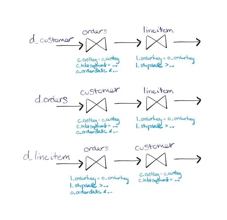
Notice how while the first two paths look similar, the third path gets to put its constraints in a different order. This new order moves as many constraints forward as it can, and the flexibility to do things differently is an important part of doing that effectively.
Update Streams?
All of the above was about handling just one batch of updates, to only one of the inputs at a time. It also presumed that we were dealing only with additions, which made the SQL for the update rule easier to write. Things become more interesting as we consider streams of arbitrary updates at many different times, where any one time may contain updates to multiple inputs. However, we are going to borrow all of the intuition up above in determining what to do.
Materialize is presented with update streams for customer, orders, and lineitem, and needs to build a dataflow that produces an output update stream for their join. Let's start with the ideas from above, and see what sort of details we need to fill in.
We'll do that by building a dataflow that has an update path for each of its input relations. We'll use an as of yet unspecified join_with operator, whose implementation you will have to imagine for now.
1 | |
2 | |
3 | |
The intent of the join_with operator is that incoming updates (on the left) are matched up against accumulated results (the named argument to join_with), "just like" they would with the SQL queries up above. Specifically, the operator matches incoming updates to only those accumulated updates present by time, and multiplies the signs of their updates so that deletions pass through correctly.
These three paths show how to respond to each of our update streams (the d_ names). The paths also reference the relations without the d_ prefix, which is meant to be the accumulations of those update streams. That is, we could replace orders with a fragment d_orders -> accumulate. If we make those replacements, the three paths up above are defined only in terms of d_customer, d_orders, and d_lineitem, which are the update streams we receive as inputs. If we merge all of the path outputs together, we get an update stream for the whole join, which we hope reflects all of the input changes.
Now, does it actually do the right thing? Mostly. There is a nit that we'll sort out that has to do with concurrent updates to the three inputs. We'll spec out the join_with operator more clearly later, and dive in to a correction that resolves the issue. But it is largely correct, for the reason that it tracks our math up above.
So that's a dataflow we can build. But should we?
This dataflow plan has a number of join_with operators that is quadratic in the number of inputs. Each of these operators seems to need to maintain some indexed data, that accumulate mentioned up above, a whole collection's worth of maintained data. Are we maintaining multiple copies of each input relation? Is this perhaps many more than we can afford to maintain?
Naively, yes.
This approach can be pretty terrible if each of the join_with operators maintains their own indexed representation of the relation they perform lookups into. In many streaming systems, this is how the operators have to work. In these systems each operator is responsible for its own state, and this dataflow plan would be unworkably expensive in terms of memory requirements, as the number and accumulated size of the join inputs increase.
Materialize is fundamentally different in that it can share indexed representations of accumulated updates between multiple operators, and across multiple dataflows. There is a neat paper to read on the underlying technology: shared arrangements. The dataflow plan above costs only in proportion to the number of distinct indexed representations, rather than the number of uses of those representations. A "distinct indexed representation" is determined by 1. an input stream of updates, and 2. some columns on which we build an index.
So how many distinct indexed representations are there in one of these join plans?
In many standard relational settings, relational joins are done on the basis of keys. A relation's primary key is a set of columns whose values uniquely determine a row in the relation. A relation's columns may also contain foreign keys, which are references to the primary keys of other relations. It is very common for the joins to be primary-foreign key joins, where a foreign key in one relation is used to "look up" the corresponding entry in a relation with that primary key. This is the case in our example above with customer, orders, and lineitem, and it is very common in relational workloads.
In this standard setting, it is sufficient to have indexes on the primary and foreign keys for each relation. That set of distinct indexed representations that is often sufficient.This set is also often linear in the number of relations; both a star schema and a snowflake schema have one primary key for each relation, each of which has one corresponding foreign key in some other relation. Each relation then contributes at most two indexes: its own primary key index, and the foreign key index of the relation that references it.
Things can certainly get more complicated than this, but these joins cover the vast majority of what folks are writing with SQL.
Connecting the dots
These dataflows, based on the update rules we saw above, compute and maintain multiway relational joins. Materialize only needs to maintain distinct indexes, through the magic of shared arrangements. In particular, if the indexes for a dataflow already exist, no new indexes need to be built and maintained. These dataflows spend resources (compute, memory) only to move updates along the dataflow,
Conclusions
Materialize has access to join plans that are very inefficient in other streaming systems (those that cannot share indexed state). These join plans require no new arranged data when the standard indexes are in place. This dramatically reduces the costs of these plans, removing the memory costs of storing the data and the computational costs of keeping the data up to date. Best of all, these indexes are the natural ones you might expect to form in a standard relational database; no wild new concepts required!
Joins are one of the key features in Materialize. We've worked hard to lay the foundations for efficient join execution, so that the system itself doesn't need to work hard when you issue those join queries, nor when their inputs start changing and we need to keep the results up to date.
Come and talk with us on Slack if you’re interested in learning more about how Materialize works, and if this sounds like something you’d like to work on, we’re hiring!