Replace a microservice with a SQL query
tl;dr Using Materialize, you can easily create transformation-oriented microservices.
Microservices, at their best, are services that represent some conceptually small unit of work in a pipeline—maybe provisioning some new resources, or performing a transformation.
When creating microservices that operate on large datasets, teams often rely on
a job scheduler to handle incoming data in batches. These tools range from the
very basic (e.g. cron) to the very byzantine.
However, with Materialize, you can instead cut out the notion of scheduling and jobs entirely. Instead, you simply send data to Materialize, describe its transformations with SQL, and read results on the other side. And, as a bonus, it can maintain the results of your transformations with sub-second latencies, enabling newer and more nimble services.
Overview
In this demo, we’ll take the role of a VM provider, and build a microservice to produce our customers' billing data. To do this, we’ll aggregate our users' billing data based on:
- Events emitted from their running VM instances
- An updatable stream of billing information for different VM types.
In the rest of this section, we’ll cover the “what” and “why” of our proposed deployment using Materialize to provide a job-less microservice.
Events
Events in this demo represent our customers' billable actions—in this case, some amount of CPU usage over an interval of time.
We’ve chosen to represent events as
protobuf
messages, which need to include the following details:
- VM type (so we know the billable rate)
- Processing units consumed (so we know the billable units)
- Units of time (so we can create bills for different periods of time)
Pricing data
To remove complexity from this demo, we’ll keep our prices the same, and simply read them into Materialize once. However, in a production deployment, one could create another service that analyzes VM usage and dynamically sets the price.
Stream
To ferry data from our machines to our microservice, we’ll send the messages on a stream—namely, Kafka.
Materialize
Materialize itself does the bulk of the work for our microservice, which includes:
- Ingesting and decoding
protobufmessages. Note thatprotobufsources currently only support append-only writes to Materialize. In the case of event logging, append-only writes are perfectly acceptable. - Normalizing data
- Performing arbitrary transformations on data from streams, including joins and aggregations. In our case, we’ll be joining users' compute events with our billing data.
Diagram
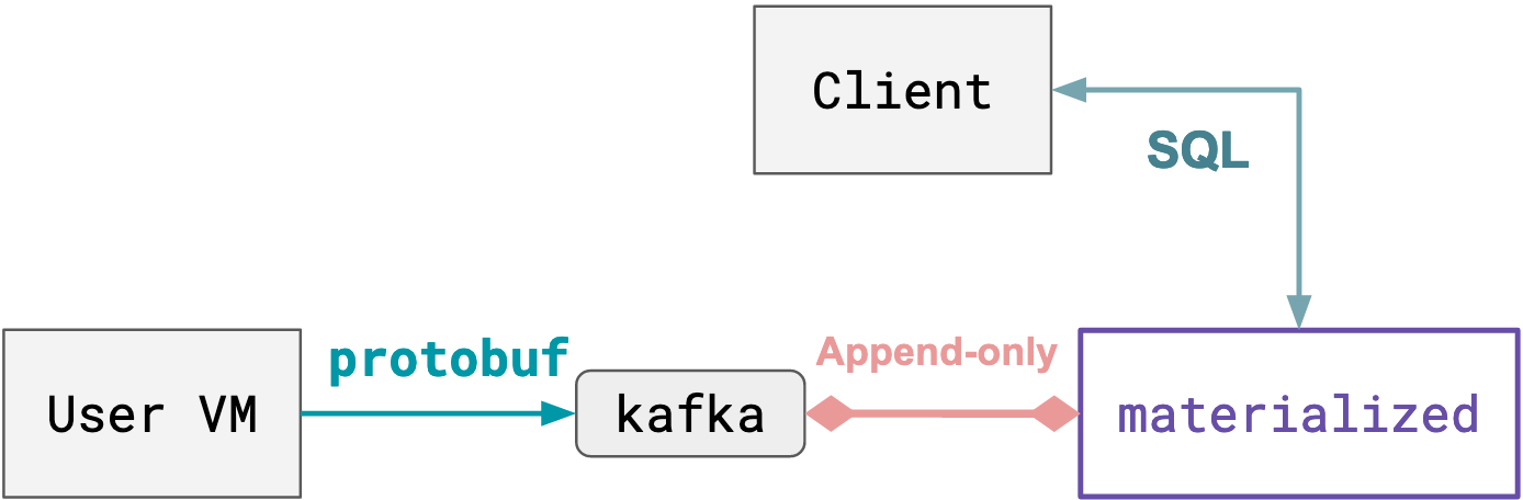
Conceptual overview
This demo includes everything you need to see a billing microservice in action, but in this section, we’ll cover the the thinking behind how the load generator was created, and provide a kind of template you could use for similar systems.
- Structure your
protobufmessages, and start emitting them. - Create a source from the stream of
protobufmessages. - Normalize our
protobufdata. - Create aggregations of our data.
Structuring messages
In this demo, we’ll rely on protobuf to format the messages we send from our
machines to the Materialize microservice. You could achieve the same thing with
Avro-encoded messages, but we wanted to highlight protobuf support.
Here’s a view of the protobuf schema we decided on:
// Details about the resource the user's consuming
message ResourceInfo {
  int32 cpu_num = 1;    // Number of CPUs
  int32 memory_gb = 2;  // Memory in GB
  int32 disk_gb = 3;    // Storage in GB
  int32 client_id = 4;  // ID of owner
  int32 vm_id = 5;      // VM's ID
}

// Some usage of the resource spanning some interval,
// identified by meter and measured by value
message Record {
  string id = 1;             // Record's ID

  google.protobuf.Timestamp interval_start = 2; // Interval's start
  google.protobuf.Timestamp interval_end = 3;   // Interval's end

  string meter = 4; // What's being measured
  int32 value = 5; // Quantity measured

  ResourceInfo info = 6; // Resource for this Record.
}

// A collection of Records over a contiguous interval
message Batch {
  string id = 1;             // Batch's ID

  google.protobuf.Timestamp interval_start = 3; // The start of the earliest record
  google.protobuf.Timestamp interval_end = 4;   // The end of the latest record

  repeated Record records = 7; // Records in Batch
}
If you aren’t familiar with protobuf here’s a quick overview:
messagefields are structured asrepeated? type field_name = field_id.repeatedindicates that the field is equivalent to a vector.field_idis an immaterial implementation detail for this demo, so don’t worry too much about it.
The nested structure of Batch is denormalized, which can make it challenging
to use within a relational system, like Materialize. However, we can nicely
normalize the data at a later point, so we don’t need to change anything from
the perspective of our events.
From here, we’ll start publishing these messages on a Kafka topic.
Create a source from our protobuf messages
protobuf sources in Materialize require the following pieces of information:
| Requirement | Purpose | Demo value |
|---|---|---|
| Source URL | Where to listen for new messages (hostname/topic_name) |
kafka://localhost/billing |
| Schema | How to decode messages | Generated FileDescriptorSet |
| Message name | The top-level message to decode | billing.Batch |
Generating protobuf schema/FileDescriptorSet
To decode protobuf messages, we need to know the messages' schema (known as a
FileDescriptorSet), which you can generate from protoc.
Assuming you are in the directory alongside your .proto files:
protoc --include_imports --descriptor_set_out=SCHEMA billing.proto
This generates a FileDescriptorSet file named SCHEMA.
The --include_imports flag is important if your .proto file imports from any
other files; it transitively imports all imported message descriptors. In our
example, it doesn’t do anything, but in a production-grade example, you’re
likely to need it.
Creating a protobuf source
Now that we have the FileDescriptorSet, we can generate a protobuf source:
CREATE SOURCE billing_source
FROM KAFKA BROKER 'localhost:9092' TOPIC 'billing'
FORMAT PROTOBUF MESSAGE 'billing.Batch'
    USING SCHEMA FILE '[path to schema]';
Normalizing data
The data we receive from the new billing_source needs to be normalized from its original structure.
In Materialize, we can accomplish this with a materialized view:
CREATE MATERIALIZED VIEW billing_records AS
    SELECT
        (r).id,
        id batch_id,
        to_timestamp(((r).interval_start)."seconds")::text interval_start,
        to_timestamp(((r).interval_end)."seconds")::text interval_end,
        (r).meter,
        ((r)."value")::int,
        ((r).info).client_id::int,
        ((r).info).vm_id::int,
        ((r).info).cpu_num::int,
        ((r).info).memory_gb::int,
        ((r).info).disk_gb::int
    FROM
        billing_source,
        unnest(records) as r;
This makes billing_records a normalized view of our data that we can begin
writing queries from. Here’s its schema:
SHOW COLUMNS FROM billing_records;
     name       | nullable |    type
----------------+----------+--------------------------
 id             | t        | text
 batch_id       | t        | text
 interval_start | t        | timestamp with time zone
 interval_end   | t        | timestamp with time zone
 meter          | t        | text
 value          | t        | integer
 client_id      | t        | integer
 vm_id          | t        | integer
 cpu_num        | t        | integer
 memory_gb      | t        | integer
 disk_gb        | t        | integer
(11 rows)
Other source types
As we mentioned before, it’s also possible to create a stream of pricing
information that uses protobuf messages similar to our events. However, for
simplicity, we’ve decided to create a simple file for our pricing data.
For our demo’s pricing data, we’ll just keep a CSV of client IDs and the prices
they pay per second with the format (client_id, price_per_cpu_second, price_per_gb_second)
Here’s an example of what our pricing data looks like:
1, 3, 6
2, 2, 3
3, 1, 7
4, 4, 3
And here is how we can import that into Materialize.
CREATE SOURCE price_source
FROM FILE 'prices.csv'
FORMAT CSV WITH 3 COLUMNS;
This creates a source with the following columns:
    name    | nullable |  type
------------+----------+--------
 column1    | f        | text
 column2    | f        | text
 column3    | f        | text
 mz_line_no | f        | bigint
We’ll then create a materialized view for this data, as well as convert its units from seconds to milliseconds. This isn’t strictly necessary because we could just SELECT from pricing_source, but is more performant in our case.
CREATE MATERIALIZED VIEW billing_prices AS
    SELECT
        CAST(column1 AS INT8) AS client_id,
        ((CAST(column2 AS FLOAT8)) / 1000.0)
            AS price_per_cpu_ms,
        ((CAST(column3 AS FLOAT8)) / 1000.0)
            AS price_per_gb_ms
    FROM price_source;
For more details on how CSV sources work, see CREATE SOURCES.
Aggregating data
Now that we have both the pricing and usage data, we can start generating useful reports about our customers' usage to determine their billing.
Let’s determine their monthly usage by resource type. Note that our notion of
“resource type” is slightly denormalized because we define it by a collection of
properties (cpu_num, memory_gb, disk_gb), but don’t explicitly define that
these columns have a relation, even though they do.
CREATE MATERIALIZED VIEW billing_agg_by_month AS
    SELECT
        substr(interval_start, 0, 8) as month,
        client_id,
        meter,
        cpu_num,
        memory_gb,
        disk_gb,
        sum(value)
    FROM billing_records
    GROUP BY
        month,
        client_id,
        meter,
        cpu_num,
        memory_gb,
        disk_gb;
This gives us the following columns:
| Column | Meaning |
|---|---|
month |
The month to bill |
client_id |
Unique identifier for the client |
meter |
The name of the item being billed |
cpu_num, memory_gb, disk_gb |
Identifies machine type |
sum |
The total number of metered units to bill |
Important to note is that this table shows the customers' itemized usage, i.e. their usage of distinct CPU configurations.
From here, we can simply JOIN the two tables to compute our customers' bills.
CREATE VIEW billing_monthly_statement AS
    SELECT
        billing_agg_by_month.month,
        billing_agg_by_month.client_id,
        billing_agg_by_month.sum AS execution_time_ms,
        billing_agg_by_month.cpu_num,
        billing_agg_by_month.memory_gb,
        floor(
            (
                billing_agg_by_month.sum
                * (
                        (
                            billing_agg_by_month.cpu_num
                            * billing_prices.price_per_cpu_ms
                        )
                        + (
                            billing_agg_by_month.memory_gb
                            * billing_prices.price_per_gb_ms
                          )
                    )
            )
        )
            AS monthly_bill
    FROM billing_agg_by_month, billing_prices
    WHERE
        billing_agg_by_month.client_id = billing_prices.client_id
        AND billing_agg_by_month.meter = 'execution_time_ms';
Note that there is an implicit JOIN with:
WHERE billing_agg_by_month.client_id = billing_prices.client_id
For each VM configuration, this view takes the user’s monthly usage of that VM configuration (billing_agg_by_month.sum), and multiplies it by the sum of:
- The customer’s price per CPU * the VM configuration’s number of CPUs
- The customer’s price per GB of memory * the VM configuration’s GBs of memory
Like the billing_agg_by_month view, this view shows the itemized bill.
We can also use this itemized bill to generate users' total bills:
SELECT month, client_id, sum(monthly_bill) AS total_bill
FROM billing_monthly_statement
GROUP BY month, client_id;
And that’s it! We’ve converted our protobuf messages into a customer’s monthly
bill.
Naturally, in a full-fledged deployment, you would also need a service that collects these results from the Materialize-backed billing microservice, and then actually bills your customers.
Run the demo
Our demo actually takes care of all of the above steps for you, so there’s very little work that needs to be done. So in this section, we’ll just walk through spinning up the demo, and making sure that we see the things we expect. In a future iteration, we’ll make this demo more interactive.
Preparing the environment
-
Set up Docker and Docker compose, if you haven’t already.
-
Clone the Materialize demos GitHub repository and checkout the
ltsbranch:git clone https://github.com/MaterializeInc/demos.git git checkout ltsYou can also view the demo’s code on GitHub.
-
Download and start all of the components we’ve listed above by running:
cd demos/billing
docker-compose up -d
Note that downloading the Docker images necessary for the demo can take quite a bit of time (upwards of 3 minutes, even on very fast connections).
If the command succeeds, it will have started all of the necessary infrastructure and will have generated ~1000 events.
Understanding sources & views
Now that our deployment is running (and looks like the diagram shown above), we
can see that Materialize is ingesting the protobuf data and normalizing it.
-
Launch a
psqlshell connected tomaterialized:docker-compose run cli -
Show the source we’ve created:
SHOW SOURCES;name ---------------- billing_source price_source -
We’ve also created a materialized view that stores a verbatim of all of the messages we’ve received,
billing_raw_data.We can query this view to see what our denormalized data looks like:
SELECT records FROM billing_raw_data LIMIT 1;records ----------------------------------------------------------------------------------------------------------------------------- {"(43e0b30b-0022-4a90-9594-1977e8dce33a,\"(1632335022,0)\",\"(1632335121,0)\",execution_time_ms,44,\"(2,8,128,22,1375)\")"} -
Now, we can see what our normalization looks like (the
billing_recordsview we created in the Normalizing data section):SELECT * FROM billing_records LIMIT 1;id | batch_id | interval_start | interval_end | meter | value | client_id | vm_id | cpu_num | memory_gb | disk_gb ------------------------+------------------------+-------------------------------------+-------------------------------------+-------------------+-------+-----------+-------+---------+-----------+--------- AkrKbvQ8mOMt64WHAEQw | vB_PDgD_SWm8rG0pxCsa4w | 2020-01-28T10:36:03.331566645+00:00 | 2020-01-28T10:43:41.331566645+00:00 | execution_time_ms | 32 | 12 | 1771 | 1 | 16 | 128Note that this data is very wide, so you’ll need to scroll left-to-right to view all of it.
For a more sensible view of just the schema, you can use
SHOW COLUMNS. -
With all of this data, we can start generating monthly aggregations of our customers' usage––which, remember, is just the materialized view we created in the Aggregating data section.
Let’s take a look at our top 5 highest-use customers:
SELECT * FROM billing_agg_by_month ORDER BY sum DESC LIMIT 5;month | client_id | meter | cpu_num | memory_gb | disk_gb | sum ---------+-----------+-------------------+---------+-----------+---------+------- 2021-09 | 16 | execution_time_ms | 1 | 16 | 128 | 25330 2021-09 | 86 | execution_time_ms | 1 | 16 | 128 | 24587 2021-09 | 38 | execution_time_ms | 2 | 8 | 128 | 24575 2021-09 | 97 | execution_time_ms | 1 | 16 | 128 | 24488 2021-09 | 50 | execution_time_ms | 2 | 16 | 128 | 24319 -
Now, we can look at our customers' monthly bills by selecting from
billing_monthly_statement:SELECT * FROM billing_monthly_statement ORDER BY monthly_bill DESC LIMIT 5;month | client_id | execution_time_ms | cpu_num | memory_gb | monthly_bill ---------+-----------+-------------------+---------+-----------+-------------- 2021-09 | 51 | 22709 | 2 | 16 | 3542 2021-09 | 93 | 22134 | 2 | 16 | 3541 2021-09 | 58 | 23555 | 2 | 16 | 3533 2021-09 | 89 | 21936 | 2 | 16 | 3509 2021-09 | 55 | 22352 | 2 | 16 | 3486 -
We an also perform arbitrary
SELECTs on our views to explore new aggregations we might want to materialize with their own views. For example, we can view each user’s total monthly bill:SELECT month, client_id, sum(monthly_bill) AS total_bill FROM billing_monthly_statement GROUP BY month, client_id;
Recap
In this demo, we saw:
- How to create a
protobufsource - How Materialize can normalize JSON blobs
- How to define sources and views within Materialize
- How Materialize can aggregate and transform data