Building Differential Dataflow from scratch

Differential Dataflow is a framework that lets users define a computation using functional operations like map/join/reduce/etc, and then send the computation inputs and modify the inputs, and sit back and watch the output and corresponding modifications to the outputs roll in. Differential will produce modifications to the outputs efficiently, without recomputing everything from scratch, and importantly, Differential will do this even when the computation has recursion. This post will explain Differential Dataflow by starting from scratch and reimplementing it in Python. Differential Dataflow is carefully engineered to run efficiently across multiple threads, processes, and/or machines, but we will skip all of that. We’ll also skip as much as possible the work that the Timely Dataflow layer does that’s not essential to Differential. This post will answer “what the heck is Differential Dataflow, what does it do, and why is that hard” for folks who have absolutely no familiarity with dataflow programming, Timely, or Rust, but they do have to know some Python.

Other related resources for learning about Differential include official documentation, Frank’s blog posts introducing Differential, and Jamie Brandon’s dida which is an implementation of Differential Dataflow in Zig.

Structure of this post

We’ll build up Differential in six steps starting from a small implementation that doesn’t support modifying input data at all, all the way through to the final implementation that supports any computation/any inputs (hopefully!) that the Rust implementation supports.

The blog post will focus on the high level challenges at each step and will omit some implementation details along the way to keep things moving.

v0: Intro / What are we trying to compute?

This implementation lays out the core data structure (collections), and the operations that can be performed on it. We’re establishing a baseline, so we won’t worry about collections changing for now.

We will represent data as multisets extended to allow positive and negative multiplicities^{negative-multiplicities} of immutable, typed, records. We will call these multisets collections. Collections are also themselves immutable. We’ll implement collections as a list of pairs of (record, multiplicity), where multiplicity is a (potentially negative) integer indicating how many times record is present in the collection. So as an example:

[('cat', 4), ('dog', 2)]

is a collection with 4 instances of 'cat' and 2 instances of 'dog'.

[((2, 'prime'), 1), ((2, 'even'), 1), ((3, 'prime'), 1), ((3, 'odd'), 1) ((4, 'composite'), 1), ((4, 'even'), 1), ((5, 'prime'), 1), ((5, 'odd'), 1)]

is a collection where each record is a pair of (int, str) where the first element is an integer between 2 and 5, and the second element is a string indicating whether the first element is even / odd, or prime / composite. Collections where the records are pairs have a special significance sometimes, and the first element of the pair is called a key, and the second element is called a value.

The following collections are all logically equivalent, even though physically the underlying lists are different.

[('cat', 4), ('dog', 2)]
[('cat', 1), ('cat', 3), ('dog', 2)]
[('dog', 2), ('cat', 4)]
[('cat', 4), ('dog', 2), ('elephant', 0)]
[('cat', 4), ('dog', 2), ('elephant', -4), ('elephant', 4)]

This flexibility is desirable because some operations can remain performant, and not have to worry about normalizing data or getting rid of records with 0 multiplicity. Operations that need access to normalized and deduplicated data are still free to normalize when they need to.

Finally, multiplicities in a collection can also be negative, so the following is also a valid collection.

[('apple', 2), ('banana', -2)]

Allowing negative multiplicities is important because it allows for the multiset difference between two collections to also be a collection. If we had the following two collections:

a = [('apple', 3), ('banana', 2), ('coconut', 7)]
b = [('apple', 1), ('banana', 4), ('coconut', 7)]

Then the difference between a and b is [('apple', 2), ('banana', -2)]. Differences will be more important in the next section.

We’ll be working exclusively with collections, and applying functional operations to them. Each operation will take as input one or two collections and produce a new collection as output. Some operations are summarized below, but everything is implemented in v0

• concat: combine two collections into one. concat is the same as adding two collections together. concat is also an excellent example of where the flexibility in how we are allowed to represent collections pays off as the implementation can copy the elements in both lists together into one list and not have to do any other work.

  python

  copy code

  copied successfully

  collection_a.concat(collection_b) # Compute a + b

  is analogous to collection_a UNION ALL collection_b in SQL.

• negate: multiply all multiplicities by -1. concat and negate together let you subtract collections.

  python

  copy code

  copied successfully

  collection_a.concat(collection_b.negate()) # Compute a - b

  is analogous to collection_a EXCEPT ALL collection_b in SQL.

• map / filter: apply a function f to all records in the collection and produce a new collection containing f(record) / record if f(record) == True respectively.

• reduce: this operation requires key-value structure. For each key in the input collection, reduce applies a function f to the multiset of values associated with that key, and returns a collection containing (key, f(values associated with key)). There’s a couple of operations built on top of reduce, of which a few important ones are:

  • count: return the number of values associated with each key, analogous to SELECT COUNT(val) FROM ... GROUP BY key in SQL.
  • sum: return the sum of the values associated with each key, analogous to SELECT SUM(val) FROM ... GROUP BY key in SQL.
  • distinct: return the distinct set of values associated with each key, analogous to SELECT DISTINCT(val) FROM ... GROUP BY key in SQL.

• consolidate: produce a normalized logically equivalent version of the input collection containing exactly one instance of each record, and no records with multiplicity 0.

• join: takes two input collections, and for all (x, y) in the first collection, and all (x, z) in the second collection, produces (x, (y, z)) as output. join is analogous to NATURAL JOIN in SQL.

• iterate: this operation might be surprising for most folks. iterate takes one input collection and repeatedly applies a function f to the input until the output stops changing. f can be any combination of the functional operations defined above, including other nested calls to iterate.

These functional operations (and a few more) are the verbs in Differential. All computations have to be expressed as a combination of some input collection(s) + some combination of operations applied to the input(s). The output for all computations is an output collection. As an example, we could have the following silly computation that takes a collection of numbers, repeatedly increments the numbers and adds new numbers less than six to the output, and then produces (number, number^2) for all the elements in the output. This is a demo of how all the pieces fit together and not an interesting computation in itself. We define the computation like this:

def add_one(collection):
    return (
        # Increment all records in the input.
        collection.map(lambda data: data + 1)
        # Recombine the incremented records with the original input.
        .concat(collection)
        # Keep only the records <= 5.
        .filter(lambda data: data <= 5)
        # Give the data key-value structure.
        .map(lambda data: (data, ()))
        # Compute the distinct set of records. Without this step we won't
        # halt because the collection will keep adding copies of previously
        # added records.
        .distinct()
        # Reshape the data to get rid of key-value structure.
        .map(lambda data: data[0])
    )
collection = Collection([(1, 1)])
# Perform `add_one` on `collection` till fixpoint (the output stops changing).
result = collection.iterate(add_one)
# Produce (N, N^2) from all N in the fixpoint.
.map(lambda data: (data, data * data))
print(result)

And when run, the output is, as expected:

ruchir@local intro-differential % python3 v0/collection.py
... skipping other unrelated output ...
Collection([((1, 1), 1), ((2, 4), 1), ((3, 9), 1), ((4, 16), 1), ((5, 25), 1)]

The novel/cool thing about Differential Dataflow is that it responds to changes in the inputs and produces new outputs efficiently, even when the computation includes joins or iterates. “Efficiently” here roughly means “produces new outputs in time proportional to the size of the change in inputs * assorted logarithmic factors”. Differential also does all of this interactively, in that the inputs can be updated while computation is ongoing.

v1: Sequences of difference collections

So far, we’ve set up some machinery to define some computation f as a composition of functional operations, and if we feed in input collections to f, we’ll get an output collection out. Now, we’ll support all operations from before over changing collections by expressing a collection that changes as a sequence of difference collections.

Our key problem is that we’d like for collections to remain immutable^{why-immutable}, while at the same time, we want collections to change. We’ll achieve this by accumulating immutable state that describes the way the collection is changing, without ever modifying any of the internal data that’s been added.

So for example, if we have a collection which initially equals A0, and later morphs into A1, we can describe that behavior with the following sequence of collections:

collection_sequence = [A0, A1, ...]

If the collection keeps changing, we can just add new objects to this sequence without ever modifying the previously inserted collections.

We can also equivalently represent these changes with the following sequence of difference collections:

difference_collection_sequence = [A0, A1 - A0, ...]

where A1 - A0 is shorthand for the collection A1.concat(A0.negate()).

The two representations are logically equivalent in that we can go from one representation to another with a linear amount of computation / space. We can go from collection_sequence to difference_collection by ( pseudocode):

difference_collection_sequence[i] == if i > 0: collection_sequence[i] - collection_sequence[i - 1] else: collection_sequence[i]

Note that difference_collection_sequence[0] is implicitly collection_sequence[0] - []. In the other direction (also pseudocode):

collection_sequence[i] == sum(differences_collection_sequence[v] for all v <= i )

Whenever we perform any operation f on a collection sequence, we require that the result is identical to performing the same operation to every collection in the sequence sequentially. In code, we can write that invariant as:

f(collection_sequence) == [f(A0), f(A1), ...]

or more generally:

f(collection_sequence)[i] == f(collection_sequence[i]) for all i

This is Differential’s correctness guarantee. The equivalence between collection sequences and difference collection sequences means that, performing the same operation f on the corresponding difference collection sequence, it is required that:

f(difference_collection_sequence) == [f(A0), f(A1) - f(A0), ...]

or more generally:

f(difference_collection_sequence)[i] == if i > 0: f(collection_sequence[i]) - f(collection_sequence[i - 1]) else: f(collection_sequence[i]) for all i

From here on out in this implementation and subsequent ones, a Collection object will represent a difference collection that is part of a sequence (or related generalization). In v1, the DifferenceSequence type represents a logical collection undergoing a sequence of changes, implemented as a list of difference collections (Collection objects^{naming-is-hard}).

We chose to use a sequence of difference collections (difference_collection_sequence) rather than a sequence of collections (collection_sequence) for the following reasons:

1. If subsequent collections in collection_sequences are similar to each other, the corresponding differences will be small.

2. For many operations f, we can generate the corresponding sequence of output difference collections easily by looking at the input difference_collection_sequence. We have three different flavors of functions so far:

   1. Some functions (e.g. map) are linear, which means that, for any pair of collections A and B:

      python

      copy code

      copied successfully

      f(A + B) = f(A) + f(B)

      Linear operations can compute, f(A1) - f(A0) without having to compute f(A1), and instead directly computing f(A1 - A0), where A1 - A0 is the (hopefully small) difference collection stored in difference_collection_sequence. This is also nice because most of our operators are linear (map / filter/ negate, concat) and they don’t need to change at all to work with a sequence of difference collections.

   2. join is slightly more complex. If we have two input difference collection sequences that look like:

      python

      copy code

      copied successfully

      difference_collection_sequence_a = [A0, A1 - A0, ...]
      difference_collection_sequence_b = [B0, B1 - B0, ...]

      then we need to produce as output:

      python

      copy code

      copied successfully

      difference_collection_sequence_a.join(difference_collection_sequence_b) ==
          [A0.join(B0), A1.join(B1) - A0.join(B0), ...]

      However, we would prefer to not compute A1.join(B1). Instead, we can take advantage of the fact that join distributes over multiset addition^distribute, so:

      python

      copy code

      copied successfully

      A1.join(B1) - A0.join(B0) == (A1 - A0).join(B0) + A0.join(B1 - B0) + (A1 - A0).join(B1 - B0)

      Again, the idea is that when the changes to the two inputs (A1 - A0) and (B1 - B0) are small, we should be able to take advantage of that, and produce the respective changes to the output without having recompute the full output from scratch. Unfortunately, our flat list representation of collections leaves a lot to be desired on that front, and so we have to introduce an Index object, which stores a map from keys -> list of (value, multiplicity) so that we can perform a faster join that only takes time proportional to the number of keys changed by the input differences.

   3. reduce in general cannot take advantage of the structure of the sequence of difference collections because the reduction function might not have any friendly properties we can exploit (e.g. when calculating a median). reduce has to instead keep doing the work we successfully avoided above.

      Going in order over each collection in the input difference collection sequence (self._inner in the code), it adds the data to an Index and remembers the set of keys that were modified by that difference

      python

      copy code

      copied successfully

      for collection in self._inner:
          keys_todo = set()
          result = []
          for ((key, value), multiplicity) in collection._inner:
              index.add_value(key, (value, multiplicity))
              keys_todo.add(key)
              ...

      Then, for each key that was modified by an input difference, it accumulates all input (value, multiplicity) changes associated with that key and the current output for that key.

      python

      copy code

      copied successfully

              ...
              for key in keys_todo:
                  curr_input = index.get(key)
                  prev_out = index_out.get(key)
                  ...

      It then recomputes new values of the output from the current input and produces as output the difference between the most recent output f(curr_input) and the previous output prev_out. It finally adds that to the output difference collection sequence, and remembers the output in an Index in case the key changes again.

      python

      copy code

      copied successfully

                  ...
                  out = f(curr_input)
                  delta = subtract_values(out, prev_out)
                  for (value, multiplicity) in delta:
                      result.append(((key, value), multiplicity))
                      index_out.add_value(key, (value, multiplicity))
          output.append(Collection(result))
          index.compact(keys)
          index_out.compact(keys)

      Note that expressing inputs and outputs with difference collections doesn’t help with computing reduce in the general case^reduce, but it doesn’t hurt much either. Also, if we keep inputs and outputs indexed as we did for join, we can recompute the reduction for the subset of keys that were modified by an input instead of recomputing the reduction on the full collection.

For now, we’ll skip iterate because we don’t have the machinery to do it well. Aside from that, this implementation supports computing all other operations efficiently when the sequence of all changes to all inputs is known in advance.

v2: Constructing dataflow graphs

v2 extends the previous implementation to support performing computations in the online setting when we don’t know all changes to all inputs in advance.

The main difficulty in doing so is that previously, all of our functional operations were implemented as methods which were invoked once and would go through all of their input difference collections, and produce all outputs. We’ll instead need a way to invoke the same functional operation multiple times, as new input difference collections get added. Some functional operators need to hold on to additional state (for example, join holds on to indexes), so our implementation needs to be able to do that as well. Similarly, previously the difference collection sequences were defined once as a list with all changes. Now, they’ll need to be more like queues where new data gets added over time.

Up until this point we have been writing imperative code. We’ve been defining some variables, and telling the computer to perform various functions on that data, and give us a result back. Now, we have to more explicitly construct a dataflow graph, where the vertices correspond to our operations, and the edges correspond to data that are inputs and outputs of those operations. After we’ve constructed the dataflow graph, we get to feed it data, and watch data come out^retained.

The dataflow graph vertices are instances of the Operator class, which has input and output edges and a run function which consumes input difference collections from its input edges and produces corresponding outputs to its output edges when invoked. There are further subspecialties of Operator like {Binary, Unary, LinearUnary}Operator that help reduce code duplication and make things easier to use. Operator’s input edges are instances of DifferenceStreamReader, and each Operator has one output edge which is an instance of a DifferenceStreamWriter. DifferenceStream{Reader,Writer} are thin wrappers over the Python standard library’s deque object that support sending the same logical output to multiple downstream Operators, and prevent readers from accidentally writing. They are analogous to DifferenceSequence in the previous implementation.

We still want to make things seem imperative, and easy to use, and GraphBuilder and DifferenceStreamBuilder help achieve that. To put it all together, you first have to define a new graph:

# Start creating a new graph.
graph_builder = GraphBuilder()
# Add a new input edge to the graph.
input_a, input_a_writer = graph_builder.new_input()
# Define some computations over that input.
computation_step = input_a.map(lambda data: data + 5)
    .filter(lambda data: data % 2 == 0)
input_a.negate().concat(computation_step).debug("output")
# Finish building the graph.
graph = graph_builder.finalize()

The dataflow graph we’ve constructed can be represented visually in the following diagram:

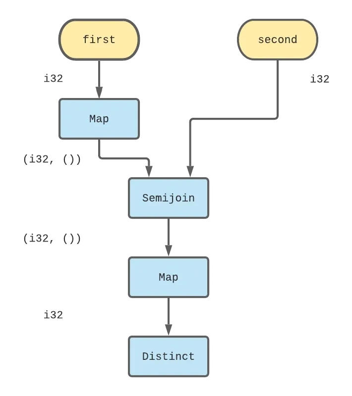
And then, you get to send the graph data, and observe results. The debug operator in this example will print its inputs to stdout.

for i in range(0, 10):
    # Send the graph a new difference collection.
    input_a_writer.send_data(Collection([(i, 1)]))
    # Tell the graph to do some work.
    graph.step()

We still can’t perform iterate, but we can support all other operations that Differential supports. This implementation has some frustrating downsides. All binary operators need to wait for a new difference collection to arrive from both inputs before they will produce any outputs, because all outputs have to be produced in order. For example, if a concat operator receives the following two sequences of inputs:

input_a = [A0, A1 - A0, A2 - A1, A3 - A2]
input_b = [B0, B1 - B0]

It can produce as output:

output = [A0 + B0, A1 - A0 + B1 - B0]

But it has to stash [A2 - A1, A3 - A2] away and wait for input_b to send more data before it will produce any more output, even though it knows with absolute certainty that they are going to be in the output in the future^anti-timely.

More generally, nothing can send partial data, or out of order data which is not good for latency. Some systems can get around this requirement by going for eventually consistent outputs. In this example, that would be like concat sending out the pending difference collections from input_a without waiting for the corresponding data from input_b. Unfortunately, because we don’t yet have a way to indicate “more data is coming, hold on”, it becomes challenging for anything downstream to interpret the output^{internal-consistency}. Fortunately, there’s a better way which we’ll get into next.

v3: Versions and frontiers

Previously, as we moved through different versions of the input, we indicated those transitions in the changes with an ordered list of difference collections. Input difference collections had integer version numbers based on their index in an underlying list, and we used that version number to determine the order of the produced output difference collections. In v3 all difference collections moving through the dataflow graph come with an explicit label denoting their version^timestamp. This gives us the flexibility to send multiple (physical) difference collections at a given version along a dataflow edge. Logically, the true difference collection at any given version is the sum of all difference collections received/sent at that version.

With this, the concat example from the previous section might receive as inputs (note that the versions are out of order):

input_a = [(version_0, A0), (version_2, A2 - A1), (version_1, A1 - A0), (version_3, A3 - A2)]
input_b = [(version_1, B1 - B0), (version_0, B0)]

And from that, the concat operator is free to produce as output, for example:

output = [(version_0, A0), (version_2, A2 - A1), (version_1, A1 - A0), (version_3, A3 - A2), (version_1, B1 - B0), (version_0, B0)]

or:

output = [(version_0, A0.concat(B0)), (version_2, A2 - A1), (version_1, (A1 - A0).concat(B1 - B0)), (version_3, A3 - A2)]

or really any other recombination / reordering of the above, so long as the slightly revised versions of the invariants we defined in v1 still hold, namely that (in pseudocode):

We can go from a sequence of collections to a sequence of difference collections:

difference_collection_sequence(version) = collection_sequence(version) - collection_sequence(version - 1)

We can go from a sequence of difference collections to a sequence of collections:

collection_sequence(version) == sum(difference_collection_sequence(v) for all v <= version)

When we apply any operation to a sequence of difference collections the results add up to what we would expect were we to apply that operation to every collection in the corresponding collection sequence from scratch.

f(difference_collection_sequence)(version) == if version > 0: f(collection_sequence(version)) - f(collection_sequence(version - 1)) else: f(collection_sequence(version)) for all versions

Really the main revision here is that we replaced brackets with parentheses to indicate that now the versions don’t correspond to indices.

This new degree of freedom to send multiple difference collections at one version adds a couple of new problems:

1. We need a way to indicate “there won’t be any more data at version v”. Previously, we didn’t worry about this because we knew we had to get exactly one difference collection at any version.
2. Our Index type needs to be able to track data received at multiple versions, so that we can receive data at versions that are not yet finished sending data, and not have that interfere with data received at prior versions.

Thankfully we have reasonable solutions here.

1. We will introduce the concept of frontiers, and send frontier updates in dataflow graph edges from one operator to another, and to/from input and output edges. A frontier of X indicates that more difference collections may be received/sent at all versions in the set [X, infinity). Equivalently, a frontier of X indicates no difference collections may be received/sent at any version less than X.

   Operators now receive messages indicating input frontier changes interspersed with input difference collections along input edges, and must send messages updating their output frontiers when they are done producing outputs at a given version. Operators have leeway in how frequently they send output frontier updates - they are not obliged to, for example, send an output frontier update for each input frontier update they receive. But they have to send an output frontier update eventually or risk stalling the computation. Similarly, users sending data along input edges also have to at some point send a frontier update indicating that some version(s) of the input are complete, or risk stalling the computation.

   This approach is similar to that taken by Timely Dataflow, in that dataflow operators receive explicit notification when some versions are complete. However, this approach is a lot simpler than timely’s and there is no central scheduler that knows about the structure of the overall graph and is tracking progress as things change^{compare-to-timely}. Operators reason locally about their individual progress, and are obligated to eventually notify their downstream peers of it eventually, and that’s it.

2. Index has to become version aware and become a multiversion index, or more specifically, a map from key -> versions -> list of values. This is roughly analogous to arrangements in the Rust implementation^arrangements.

With these changes we can modify all operators implemented so far to work with versions.

All unary linear operators are able to produce outputs at versions before they are completed. Nothing really changes for them, they just read in their input (version, difference_collection)s, produce f(difference_collection) and happily add (version, f(difference_collection)) to their outputs. They forward along any frontier updates they receive at their input to their output.

concat receives (version, difference_collection)s from both inputs and forwards them all unchanged to its output. It tracks the min input frontier across both inputs, and updates its output frontier when the minimum changes.

join receives (version, difference_collection)s from both inputs, and produces an output at max(difference_collection_version, stored_index_version) when it finds two records with a matching key in an input and a previously indexed record. Like concat, join also tracks the min input frontier across both input edges and updates its output frontier when that min input frontier changes. join also compacts its stored indexes at that point.

reduce/consolidate need^clarify-need to wait for their inputs to stop sending data at a version before producing output at that version. Once the input frontier advances and a version is closed, consolidate does as required and produces a single consolidated difference collection at that version. reduce as before, accumulates all inputs received up to that version, and recomputes the reduction function, and then subtracts from that the output produced up to that version. reduce has to additionally be careful to compute outputs in order - so for example, if versions 0, 1 and 2 are closed with one notification indicating that the new input frontier is 3, reduce must first produce the output for 0, then 1, and then finally 2, to ensure that the output difference collection adds up correctly.

The big missing piece of the puzzle now is iterate. Let’s think about what we’d like to happen when we iterate.

Let’s say we have some collection called A (not a difference collection, just a vanilla static collection like in v0). As we perform some computation f, we’d like to produce:

iterate_collections = [(0, f(A)), (1, f(f(A))), (2, f(f(f(A)))), (3, f(f(f(f(A))))), ...]

Which looks like something we should be able to do, because that’s a sequence of collections, and we can express that with a sequence of difference collections, like:

iterate_difference_collections = [(0, f(A)), (1, f(f(A)) - f(A)), (2, f(f(f(A))) - f(f(A))), (3, f(f(f(f(A)))) - f(f(f(A)))), ...]

But if A is itself a sequence of difference collections:

A = [(0, A0), (1, A1 - A0), (2, A2 - A1), ...]

then we need to produce something like a sequence of sequences of difference collections, one for each version of A. Unfortunately, we don’t yet have a good way to specify what version for example, the difference collection produced at, say the fifth iteration of computing f on the 10th version of A should land on, and without a version to label a difference collection, we can’t really do anything. We’ll sort that out in the next section.

v4: Multidimensional versions

In v4 we extend the version type to support versions that are integer tuples ordered lexicographically. We can then use integer tuple versions to represent (toplevel_input_version, iteration_count), so from the example above, the fifth iteration of computing f on the 10th version of an input A would produce output at version (10, 5). We’ll use this to finally perform iterative computations on inputs as they change.

Lexicographic ordering on tuples of equal length basically means that tuple_a is less than tuple_b if the first element where the two differ when going from left to right, is smaller in tuple_a than in tuple_b. In Python, the corresponding comparison function could look like:

# Return true if tuple_a <= tuple_b wrt lexicographic order.
def less_equal(tuple_a, tuple_b):
    assert len(tuple_a) == len(tuple_b)
    for (a, b) in zip(tuple_a, tuple_b):
        if a < b:
            return True
        if b < a:
            return False
    return True

We don’t have to write this comparator because this is Python’s default when comparing tuples. Note that this ordering is still, like comparing integers, totally ordered. The correctness invariants are all still exactly the same. In fact, nothing really changes for any of the operators, and nothing has to change in any of the operator implementation code.

Now we’re ready to talk iteration. We need to take a difference collection sequence and slap another coordinate onto the version. We’ll use that coordinate to track changes across iterations. So for example, if we have the following data / frontier updates coming through an input dataflow edge:

input_a = [(0, A0), (Frontier(1)), (1, A1 - A0), Frontier(2), (2, A2 - A1), ...]

where Frontier(x) is a way to express that the frontier advanced to x. We’ll need to turn that input into something that looks like:

input_a = [((0, 0), A0), (Frontier((1, 0))), ((1, 0), A1 - A0), Frontier((2, 0)), ((2,0), A2 - A1), ...]

We want to produce something that looks like, for each of these inputs differences, for example A0:

output = [((0, 0), f(A0)), ((0, 1), f(f(A0)) - f(A0)), ((0, 2), f(f(f(A0))) - f(f(A0))) ...]

until the output stops changing. We don’t quite know how to produce this output yet however. We can think backwards, and ask: “what inputs would produce this output?“. Said a different way, this output comes as a result of applying f to a difference collection sequence. This output also represents the sequence of collections (not differences, but aggregated up):

output_collection_sequence = [((0, 0), f(A0)), ((0, 1), f(f(A0))), ((0, 2), f(f(f(A0)))) ...]

So the corresponding input_collection_sequence to produce this output must be (again not differences, but aggregated up):

input_collection_sequence = [((0, 0), A0), ((0, 1), f(A0)), ((0, 2), f(f(A0))) ...]

And the key things to note now are that we already have the first element in this sequence, and otherwise:

input_collection_sequence((v, i)) == output_collection_sequence((v, i - 1)) for all v; i > 0

All of this to say, we can forward the outputs we produce back to the input at the next loop iteration index, and that should be sufficient to produce the next required output^semi-naive. However, we need to be a bit careful because if we just add the output difference collection sequence back to the input after forwarding, we get an input that looks like:

input + forwarded_output_difference_collection_sequence =
    output = [((0, 0), A0), ((0, 1), f(A0)), ((0, 2), f(f(A0)) - f(A0)), ((0, 3), f(f(f(A0))) - f(f(A0))) ...]

This is not actually correct because now there’s an extra A0 at every version != (0, 0). So we need to subtract out the extra A0 at (0, 1)^impulse.

To recap the whole picture, we have to take the following steps:

1. We need to take our input difference collection sequence, and extend its version type to add a new iteration count index. We need to convert

   python

   copy code

   copied successfully

   input_a = [(0, A0), Frontier(1), (1, A1 - A0), Frontier(2), ...]

   Into:

   python

   copy code

   copied successfully

   input_a_entered = [((0, 0), A0), Frontier((1, 0)), ((1, 0), A1 - A0), Frontier((2, 0)), ...]

2. We need to retract the inputs at the second (1th) iteration, so our input sequence also needs to contain:

   python

   copy code

   copied successfully

   input_a_entered_negated = [((0, 1), A0.negate()), ((1, 1), (A1 - A0).negate()), ...]

3. As we generate output, we need to feed it back to the input at version corresponding to the next loop iteration. As we repeatedly perform f our output might be:

   python

   copy code

   copied successfully

   output = [((0, 0), f(A0)), Frontier((0, 1)), ((0, 1), f(f(A0)) - f(A0)), Frontier((0, 2)), ((0, 2), f(f(f(A0))) - f(f(A0))) ...]

   and we can concatenate it back to the input as:

   python

   copy code

   copied successfully

   feedback = [((0, 1), f(A0)), Frontier((0, 2)), ((0, 2), f(f(A0)) - f(A0)), Frontier((0, 3)), ((0, 3), f(f(f(A0))) - f(f(A0))) ...]

4. Eventually the computation has to reach a fixed point, although that’s not really our responsibility.

5. Finally, we need to communicate our results back to other downstream operators. We’ll need to truncate the timestamps back from the output to produce:

   python

   copy code

   copied successfully

   external_output = [(0, f(A0)), Frontier(0), (0, f(f(A0)) - f(A0)), Frontier(0), (0, f(f(f(A0))) - f(f(A0))) ...]

Surprisingly, this all falls out pretty naturally and part of the reason is that - the feedback difference collection sequence, the input difference collection sequence, and the output difference collection sequence all … mostly contain the same data with some minor tweaks. All of these steps are performed in the ingress, egress and feedback operators and these operators are connected together in a single iterate operator. All the code is here in v4.

With all that done, we can take it for a spin! Everything about setting up the graph is the same as before:

# Start building a new dataflow graph.
graph_builder = GraphBuilder(Version(0))
# Add a new input
input_a, input_a_writer = graph_builder.new_input()

# Define a function that produces for each input record, the set
# {record * 2^0, record * 2^1, record * 2^2 ... record * 2^n} s.t.
# the produced outputs are <= 50.
def geometric_series(collection):
    return (
        collection.map(lambda data: data * 2)
        .concat(collection)
        .filter(lambda data: data <= 50)
        .map(lambda data: (data, ()))
        .distinct()
        .map(lambda data: data[0])
        .consolidate()
    )

# Iterate over the input and print outputs to stdout and connect a reader to
# the output so that we can track progress.
output = input_a.iterate(geometric_series).debug("iterate").connect_reader()
graph = graph_builder.finalize()

Once again, we can visualize the constructed dataflow graph as a diagram to get a better feel for what’s going on.

Here the large box labelled iterate all represents the one iterate operator, and the gray shaded box represents the operators that actually perform each step of the iterative computation defined by the user. The other operators inside iterate are the various bits of machinery we built up to take in inputs, send them through one step of the computation and eventually swing the outputs around as feedback.

And then we can send it some input data, and sit back and let the graph do its work:

input_a_writer.send_data(Version(0), Collection([(1, 1)]))
input_a_writer.send_frontier(Version(1))

# Keep doing work until the output advances to version 1.
while output.probe_frontier_less_than(Version(1)):
    graph.step()

When run, we get as expected:

ruchir@local intro-differential % python3 v4/differential_dataflow.py
debug iterate data: version: Version((0,)) collection: Collection([(1, 1), (2, 1)])
debug iterate data: version: Version((0,)) collection: Collection([(4, 1)])
debug iterate data: version: Version((0,)) collection: Collection([(8, 1)])
debug iterate data: version: Version((0,)) collection: Collection([(16, 1)])
debug iterate data: version: Version((0,)) collection: Collection([(32, 1)])
debug iterate notification: frontier Version((1,))

We can modify the data in a subsequent version, e.g. with:

input_a_writer.send_data(Version(1), Collection([(16, 1), (3, 1)]))
input_a_writer.send_frontier(Version(2))
while output.probe_frontier_less_than(Version(2)):
    graph.step()

and observe the following additional outputs:

...
debug iterate data: version: Version((1,)) collection: Collection([(3, 1), (6, 1)])
debug iterate data: version: Version((1,)) collection: Collection([(12, 1)])
debug iterate data: version: Version((1,)) collection: Collection([(24, 1)])
debug iterate data: version: Version((1,)) collection: Collection([(48, 1)])
debug iterate notification: frontier Version((2,))

Note here that it didn’t produce any additional records for the newly inserted (16, 1). We’re being incremental!

Unfortunately, we’re not quite done yet. If we issue a retraction, for example with:

input_a_writer.send_data(Version(2), Collection([(3, -1)]))
input_a_writer.send_frontier(Version(3))
while output.probe_frontier_less_than(Version(3)):
    graph.step()

the output is not right, and we only get:

debug iterate data: version: Version((2,)) collection: Collection([(3, -1)])
debug iterate notification: frontier Version((3,))

When really we expected to see all the multiple of 3 outputs removed from the output. If you think about what happened when we first inserted (3, 1):

1. In the first round of iteration we send distinct [(3, 1), (6, 1)]. distinct produces as output [(3, 1), (6, 1)]. I’m intentionally omitting the fake value. Our output after the first round of iteration is [(3, 1), (6, 1)].
2. At the second round of iteration, we combine the output from the first round + the negation of the original input. So, the input to the second round is [(3, 1), (6, 1), (3, -1)], which is equivalent to [(6, 1)]. distinct in the second round receives as an input difference collection [(6, 1), (12, 1)], and produces as output [(12, 1)] (because 6 is already part of the distinct set). Crucially, the distinct operator has in its input index (6, 2)!
3. When we later retract 3 by sending (3, -1), distinct receives as input [(3, -1), (6, -1)]. It only produces as output (3, -1), because it still has a (6, 1) left over from the previous versions second iteration.
4. The output from the first iteration after retracting 3 is(3, -1) which gets fed back to the input, and combined with (3, 1), which is the negation of retracting 3. Those two differences cancel each other out, and we’re done.

Here’s a slightly different, more abstract way to think about all of this.

When we order inputs in lexicographic order, we are sending the iteration subgraph the following sequence of differences:

[A0, f(A0) - A0, f(f(A0)) - f(A0), f(f(f(A))) - f(f(A0)), ... A1 - A0]

If we accumulate all of those inputs up almost all the terms cancel out, and we’re giving the system the input:

f^infinity(A0) + (A1 - A0)

and asking it to compute the fixedpoint of f applied repeatedly to that input, and hoping that the end result equals f^infinity(A1). Unfortunately, that’s not true for all f, and/or all potential changes (A1 - A0). As it turns out, our implementation so far can only (I think) handle monotonic computations (i.e. computations that only ever add elements to their outputs), and monotonic changes to the inputs (i.e. records are only ever added to inputs and never removed). To be honest, my understanding of the subset of computations this particular implementation supports is sketchy at best^alice-book.

However, we don’t want to limit ourselves to monotonic computations. We can fix this approach in lexicographically ordered times by implementing more correct ingress and egress operators that correctly delete all previously computed work and start from scratch at each iteration. But then we won’t actually be incrementally computing the fixedpoints as the input changes.

It would be nice if we could somehow capture “the 2nd iteration at version 1 shouldn’t be influenced by e.g. the 2nd iteration at version 0.“. At the same time, we don’t want to recompute things from scratch, and so we’d still like, for example, the 2nd iteration on version 1 to take advantage of all the sweet work we did in the 1st iteration at version 0. But we’re sort of stuck because we’re limited to remembering and using all historical versions that are less than the current versions. We’ll get unstuck finally in the next section by generalizing versions to be partially ordered.

v5/vFinal: Partially ordered versions.

We have a tension between two opposing ideas:

1. Everything we have set up so far is good at handling differences, whether from new inputs, or iterations and responding to the differences efficiently
2. All differences are versioned such that they have one/zero immediate predecessor, and one successor. You have to fold in aIl differences from all historical predecessors. It’s impossible to say for example, that version (1, 1) comes after (0, 1) but not before or after (0, 2).

We’ll address that by tweaking our versions so that they are partially ordered, instead of totally ordered.

In a totally ordered set, any two elements a and b share one of the following 3 relationships with respect to <=:

(a <= b) and not (b <= a) # a < b
(b <= a) and not (a <= b) # b < a
(a <= b) and (b <= a)     # a == b

A partially ordered set adds a 4th option with respect to <= : a and b are incomparable.

(a <= b) and not (b <= a)     # a < b
(b <= a) and not (a <= b)     # b < a
(a <= b) and (b <= a)         # a == b
not (a <= b) and not (b <= a) # a and b are incomparable.

One common example of a partial order is the product partial order which defines (i1, i2, ..) <= (j1, j2, ..) if i1 <= j1 and i2 <= j2 .... We can visualize this partial order in two dimensions as points on the Cartesian plane. Here, a <= b and a <= c but b and c are incomparable. The green / blue shaded regions are all the points that are <= c and a respectively.

This partial order might be used in the real world for example, to say that a 4-hour flight that costs $350 isn’t clearly better or worse than a 6 hour $200 flight.

When we use this partial order, the difference from (version1, iteration 2) will be <= (version2, iteration2), but not (version2, iteration1). We can use this property at each (version i, iteration j) to add up all outputs produced at all (version i', iteration j') where i' <= i and j' < j. Since we no longer have sequences of difference collections, we’ll follow Differential’s lead and call a set of collections/difference collections over a partially ordered set of versions a collection/difference collection trace.

We’ll have to revisit all the places we used versions so far to make sure everything is compatible with the new, partially ordered versions. Previously:

1. We used versions to convert from collection traces to difference traces, which was necessary to accumulate inputs in the reduce operator.
2. We had to take the max of versions in join, to determine which versions various output values would be sent at.
3. We represented a frontier as a single, minimal version, and used that version to check if subsequent data was respecting the frontier, or if a frontier needed to be updated. Furthermore, we compared two frontiers to find the minimum frontier when dealing with binary operators like concat or join.
4. We used frontiers to compact data from versions where the frontier was ahead of the data version, and we forwarded the data up to the minimal version that defined the frontier.

We’ll need to make changes at all of these places.

1. Before to go from the difference trace to the actual collection trace at version v, you had to add up all the differences for all versions <= v. That’s still true, but now, the <= is the partial order <=.

   python

   copy code

   copied successfully

   collection_trace[version] = sum(differences_trace[v] for all v <= version)

   Before, the difference at version v was collection_trace[v] - collection_trace[v - 1]. Now, there isn’t a clear predecessor (what would it mean, for example, to say (6 hours, $200) - 1?), but we can still recover the difference_trace[version] by moving around terms from the expression above to get:

   python

   copy code

   copied successfully

   differences_trace[version] = collection_trace[version] - sum(differences_trace[v] for all v < version)

   Another way to visualize what’s going on is with a table. As a collection changes from A0 to A1 to A2, and so on, we receive the [A0, A1 - A0, A2 - A1, ...] as inputs, and as we apply f iteratively to those differences, we produce the following table of differences at each (version, iteration):

   	version 0	version 1	version 2
   iteration 3	...	...	...
   iteration 2	f(f(A0)) - f(A0)	f(f(A1)) - f(f(A0)) - f(A1) + f(A0)	...
   iteration 1	f(A0) - A0	f(A1) - f(A0) - A1 + A0	f(A2) - f(A1) - A2 + A1
   input	A0	A1 - A0	A2 - A1

   You can verify that, for any (version, iteration), the sum of all the differences at (v', i') <= (version, iteration) == f^iteration(A[version]) where f^iteration is just shorthand for f applied iteration times, and A[version] is the value of A at version. Also note that at any given version, the difference at iteration is just the difference at iteration - 1 with an extra f applied to every term^{why-does-this-work}.

2. We don’t have a max anymore in the partially ordered world, because not all pairs of elements are comparable to each other. But, we still have upper, bounds, where u is an upper bound of x and y if:

   python

   copy code

   copied successfully

   x <= u and y <= u

   There can be many potential z’s that serve as upper bounds for any pair of x and y, and Differential requires that there be exactly one z that is <= all the rest (alternatively, is a lower bound of all potential upper bounds), and this is called the least upper bound, and also, unfortunately in our setting, the join:

   python

   copy code

   copied successfully

   least_upper_bound(x, y) <= u for all u if x <= u and y <= u

   Partially ordered sets where all pairs of elements have a least upper bound, and analogously, a greatest lower bound are called lattices.

   max(x, y) is equal to least_upper_bound(x,y) in the one dimensional, totally ordered case. When we are specifically using the product partial order:

   python

   copy code

   copied successfully

   least_upper_bound((i1, i2, ...), (j1, j2, ...)) = (max(i1, j1), max(i2, j2), ...)

   We can again look to the two-dimensional case to get some idea for what this looks like geometrically.

   

3. Before, we could represent the set of versions that may still get new data as the interval [X, infinity), where X was the unique minimum version that might receive new data. Now, just like we don’t have max, we don’t have min either, for the same reason - not all pairs of versions are comparable. But we don’t quit. Let’s say for example, that version (0, 0) is done receiving new updates. We know there’s an infinite set of versions out there that might still receive new updates like (2, 3), or (55, 10000). We know that some versions in this set are <= other versions in this set - for example, (2, 3) < (55, 10000). Now, the set of versions that could still receive data has a set of minimal lower bounds, in this case { (1, 0), (0, 1) }. To rephrase, if all versions except for (0, 0) could receive new updates, then either (1, 0) or (0, 1) will be <= any version that receives new updates. That set is our new frontier, and it has to be an instance of an Antichain which is a set of incomparable elements (for example (0, 1) and (1, 0) are incomparable with each other). If any two elements in the antichain were comparable, we could just keep the smaller one and not lose any information.

   Instead of representing the frontier as a single minimal version, it has to now be an antichain of minimal versions. We still need to be able to a) compare a frontier with a version, to make sure that the version is allowed by the frontier, and b) compare frontiers with each other, to determine when a frontier has advanced.

   We already know how to do a). A frontier is <= a version if some element in the frontier is <= that version. For example, if we had the frontier f = Antichain([(2, 5), (4, 1)]) then f <= (3,6), because (2, 5) < (3, 6) but f <= (3, 3) is False. We can again display this situation below.

   

   Here, A and B are the elements of the antichain f, and C is the point (3, 6) (all allowed points where f <= point are shaded in green), and D is (3, 3).

   For b) an intuitive way to think about it is - every frontier describes a set of versions that could potentially get more updates, and the frontier is <= all the elements of that set. This is the set we shaded in green in the previous image. Let’s say we call that set the upper set:

   python

   copy code

   copied successfully

   upper_set(f: Antichain) = set(v in versions if f <= v)

   Two frontiers f and g can be ordered so that f <= g if:

   python

   copy code

   copied successfully

   upper_set(g).issubset(upper_set(f)) # the upper set of g is a subset of the upper set of f

   The set of all frontiers is a lattice where the greatest lower bound of two frontiers f and g has as its upper set the union of the upper sets of f and g.

   python

   copy code

   copied successfully

   upper_set(glb(f, g)) = upper_set(f).union(upper_set(g))

   We’re going to skip over some math^{subset-inclusion}, but all of this leads us to an algorithm for computing the greatest lower bound of two frontiers - take the union of all the elements in both frontiers and remove any elements that are not minimal. The important takeaway is that thinking about the upper sets induced by a frontier is an intuitive way to think about the purpose of a frontier, and can help understand the algorithms to determine whether for example, frontiers f and g satisfy f <= g.

4. Compaction: Justin Jaffray has a blog post about how Differential deals with compaction that goes over all the details. At a super high level, we previously compacted all versions <= the frontier to the minimum version allowed by the frontier. Now there isn’t a minimum version, so we cannot compact all prior versions into one, and we need to respect the fact that different future versions need access to different subsets of versions. For example (2, 4) <= (4, 4), (2, 3) <= (3, 3) but (2, 4) and (3, 3) are incomparable. If we combined (2, 4) and (2, 3) into a single version when (3, 3) could still receive updates then we might run into problems e.g. accumulating up all inputs for reduce at (3, 3). This is a rushed explanation and the linked blog post has a lot more detail.

The code to do all of these things lives in order.py, and now there’s one final wrinkle before we can think about how to do iteration. Let’s say we have a collection composed of household items, that we insert at version (0, 0) like:

[(chair, 4), (desk, 2), (towel, 5), ...]

If we apply the distinct operator to this collection, then at time (0, 0), we would observe the following output collection:

[(chair, 1), (desk, 1), (towel, 1), ...]

Now if at version (1, 0), we add the following difference collection:

[(couch, 1)]

At (1, 0) we will observe as output the new difference:

[(couch, 1)]

We can insert the same input at version (0, 1), and observe the same output: [(couch, 1)]. If we don’t do anything to course correct, at time (1, 1), the sum of all differences at times <= (1, 1) which in this case is (0, 0), (0, 1) and (1, 0) would add up to

[(couch, 2), (chair, 1), (desk, 1), (towel, 1)]

However, the correct output at time (1, 1) has (couch, 1). No sweat, at time (1, 1) we have to emit: (couch, -1) to get things to add up right. This is a bit perplexing however because:

1. There weren’t any new inputs at (1, 1).
2. We never removed anything, we only ever added household items!

This is spiritually equivalent to a merge conflict, where multiple people touch the same file, and then their changes need to be reconciled to get back to a good state. Another analogy for this is that this is kind of like the situation when someone moves in with their partner. They had a couch, which they loved. Their partner had a couch, which they also loved, but then when the two of them moved in together, suddenly one of the couches had to go. Having to emit this mysterious (couch, -1) is kind of annoying, as now in reduce we have to check all potential versions that may change their outputs on every new input, but on the much more positive side, we’re able to hold together multiple independent sources of changes, which we wanted all along!

Whew. Ok after all of that, we’re ready to go back to the example from the previous section. Everything else about all the operators/iteration is all the same.

The graph setup/sending data code is all the same except now all frontiers are Antichain objects containing a single version. When you run it, you get:

ruchir@local intro-differential % python3 differential_dataflow.py
...
debug iterate data: version: Version((0,)) collection: Collection([(1, 1), (2, 1)])
debug iterate data: version: Version((0,)) collection: Collection([(4, 1)])
debug iterate data: version: Version((0,)) collection: Collection([(8, 1)])
debug iterate data: version: Version((0,)) collection: Collection([(16, 1)])
debug iterate data: version: Version((0,)) collection: Collection([(32, 1)])
debug iterate data: version: Version((1,)) collection: Collection([(3, 1), (6, 1), (16, 1), (32, 1)])
debug iterate data: version: Version((1,)) collection: Collection([(12, 1)])
debug iterate data: version: Version((1,)) collection: Collection([(24, 1)])
debug iterate data: version: Version((1,)) collection: Collection([(16, -1), (48, 1)])
debug iterate data: version: Version((1,)) collection: Collection([(32, -1)])
debug iterate data: version: Version((2,)) collection: Collection([(3, -1), (6, -1)])
debug iterate data: version: Version((2,)) collection: Collection([(12, -1)])
debug iterate data: version: Version((2,)) collection: Collection([(24, -1)])
debug iterate data: version: Version((2,)) collection: Collection([(48, -1)])

Woohoo!! We’re finally getting the results we wanted to see!

Guarantees

Everything written so far has been really focused on maintaining a strict correctness invariant - all the output produced must exactly equal the results if the computation was performed sequentially, from scratch on each version of the input. All the operators have a mathematical definition, so ensuring correctness boils down to making sure the operator implementations are computing the right thing, and we’re always accumulating difference collections and sending out frontier updates correctly. That’s not trivial to verify, but we’ve been concerned about it from the beginning of this post.

A different flavor of guarantee that we might care about is liveness. More specifically, if we send a dataflow graph some input difference collections and advance some frontiers, we might care about:

• Progress: will the graph eventually produce the outputs, or will it hang forever?
• Termination: will the graph eventually stop producing outputs and frontier updates, or will it keep sending outputs and frontier updates forever?

We’ll sketch out the intuition for why this implementation satisfies these properties in this section. Let’s first talk about acyclic dataflow graphs (those without any iterate / feedback edges). In this setting, the progress and termination requirements turn into a set of restrictions on what operators and edges can’t do. Operators have to:

• produce a bounded number of outputs for each input. This isn’t a big restriction logically because we’ve only ever been dealing with finite collections, but it means that operators cannot send, for example [('troll', 0)] an infinite number of times. Similarly, operators cannot send an unbounded number of output frontier updates in response to any individual input frontier update.
• yield executing after a finite amount of time. In other words, each operator’s run function has to return after a bounded amount of time.
• eventually produce outputs differences in response to input differences and eventually advance output frontiers as they receive input frontier updates. Operators aren’t allowed to sit and do nothing for an unbounded amount of time.

Similarly, dataflow edges have to eventually send data sent from a source operator/user input to the intended destination operator in a finite amount of time, and are not allowed to delay sending data forever.

Roughly, any acyclic dataflow graphs where all operators and edges are subject to the restrictions above will eventually produce all outputs at all closed versions. This isn’t a formal mathematical statement, but the intuition here is that all operators will receive a finite number of inputs, and eventually produce a finite number of outputs and none of those outputs can result in any more inputs for that operator (because there are no cycles). Therefore, after a finite amount of time has elapsed, all operators should have produced their outputs stopped doing additional work. Again, this is just sketching out the intuition and this is not a formal proof.

Cyclic dataflow graphs are a bit more tricky. Termination is tricky in general because the requested computation has to eventually reach a fixedpoint on the provided inputs in order to terminate. However, if there is no fixedpoint for the computation on the provided inputs it’s totally fair for the dataflow graph to continue producing outputs forever^{turing-complete}.

Putting that aside, say we know that a given iterative computation will in fact terminate on a given input. We would know that the computation has terminated at a given version once it stops producing more output differences at that version, which is just another way to say — we know f^n(x) is the fixpoint of applying f to x because f^n(x) == f^n+1(x) == ...f^infinity(x). So our condition for knowing that an input at version v has finished iterating occurs when we no longer have any more difference collections at versions (v, _) flowing through the dataflow graph. We have a wrinkle to sort out here — some dataflow graphs might produce outputs that are logically equivalent to an empty collection, but are physically non-empty.

Consider the following example:

def example(collection):
    return (
        # Perform a sequence of two maps which together are a no-op.
        collection.map(lambda data: data + 1)
        .map(lambda data: data - 1)
        # Negate the input.
        .negate()
        # Add it back to itself, producing the empty collection.
        .concat(collection)
    )

output = input_a.iterate(example).connect_reader()
graph = graph_builder.finalize()

input_a_writer.send_data(Version(0), Collection([(1, 1)]))
input_a_writer.send_frontier(Antichain([Version(1)]))

while output.probe_frontier_less_than(Antichain([Version(1)])):
    graph.step()

This computation should converge in two iterations, regardless of the input. However, there are potential ways the graph could be executed such that it actually never converges, for example if concat is always run before any of the maps and negate then at every iteration, the feedback operator (invisible here), would send collection and collection.negate() at the next version, even though logically everything adds up to zero. The way that both the Rust implementation and this implementation work around this is by requiring that all paths from input to output inside iterate have a consolidation step (basically a consolidate operator or one of the reduce variants), that waits for all inputs to finish writing new updates to a given version, and then simplifies updates that cancel each other out.

That requirement ensures that we won’t have difference collections going through the dataflow graph at versions (v, _) even after the iteration has converged for v. The other problem we have to contend with is that we don’t want to keep sending frontier updates containing some element (v, _) that gets repeatedly incremented even after we have stopped iterating at v.

In this implementation, the feedback operator tracks all the versions at which it received a difference collection, and drops frontier elements (v, _) when it detects that it observed multiple distinct (v, _) go by in various frontier updates without any corresponding difference collections sent at those versions. The computation is a little finicky because it has to be careful to forget difference collection versions when they get closed, and it has to be careful to remove (v, _) from the frontier in such a way that all other currently iterating versions can continue iterating (for example, if the frontier was Antichain[Version((2, 1)), Version((0, 3))], and we naively removed Version((0, 3)) from that antichain, we would also lose the ability to iterate at Version((1, _)) which we may not want!). It’s all pretty workable and a fairly small amount of computation and additional state in the feedback operator.

That’s all, folks!

We covered a lot of ground, but the end result is an implementation of Differential Dataflow in about 800 LOC, which should help people get up and running with the key ideas much faster.

Obviously, the Rust implementation is a lot more careful about memory utilization and avoiding copies of data, but at a higher level, there’s a bunch of qualitatively different things that the Rust implementation does better:

• Operators are more careful to yield in a bounded amount of time, which is necessary to be responsive and avoid stalls
• There are more operators, like threshold and flat_map.
• count and sum are further optimized to make use of the fact that those operations are associative
• Frontier updates are incremental. So if the frontier changes from say:

Antichain[(1, 10), (2, 8), (4, 6), (6, 4), (8, 2)]

to:

Antichain[(1, 10), (2, 9), (4, 6), (6, 4), (8,2)]

This implementation would send the whole frontier update but the Rust implementation is smart enough to send a more compact message that says, roughly “replace (2, 8) with (2, 9)“.

• The Rust implementation uses capabilities instead of frontiers, and capabilities are a better user interface than making the user sending inputs track their own input frontier
• There’s a lot of other stuff!

Thanks Andy, Frank, Jamie, Jan, Justin, Paul, Pete and Moritz for many thoughtful comments and suggestions on earlier versions of this post.