Joins in Materialize

important
This article has been updated to reflect the latest version of Materialize. The updated post is available here.
This post is also available at my personal blog.
Materialize allows you to maintain declarative, relational SQL queries over continually changing data. One of the most powerful features of SQL queries are joins: the ability to correlate records from multiple collections of data. Joins also happen to be one of the harder things to do both correctly and efficiently as the underlying data change.
Let's walk through the ways that Materialize maintains queries containing joins!
In particular, we'll see increasingly sophisticated join planning techniques, starting from what a conventional dataflow system might do, and moving through joins that can introduce nearly zero per-query overhead. Each of the new join plans we work through represent an implementation strategy that Materialize can do that other dataflow systems will struggle to replicate.
As we move through techniques, the number of private intermediate records maintained by each query dataflows drops. We'll report all 22 TPC-H queries at the end, but here are two of the largely representative queries, and the number of additional records Materialize maintains to keep the query results up to date.
1 | |
2 | |
3 | |
4 | |
5 | |
6 | |
Each of these techniques are live in Materialize now. Each comes on-line in response to indexes that you ask Materialize to prepare. The more prepared indexes, the less per-query memory required (admittedly, the more baseline memory required as well).
At the end, we'll have a forward-looking discussion of late-materialization which can further reduce the memory requirements, in a way that currently requires user assistance (we're working on it!). Throughout, the story is that Materialize can invoke efficient join patterns from relational databases in the context of scale-out dataflow processors.
Introducing Joins
Let's take a super-simple example of an "equi-join":
1 | |
2 | |
3 | |
4 | |
5 | |
6 | |
7 | |
8 | |
9 | |
Here we have two collection of data, customer and location. We want to pick out pairs from each that match on their zip field. Although we didn't write the word JOIN, that is what happens in SQL when you use multiple input collections.
Most dataflow systems will plan this join using a relatively simple dataflow graph:

Information about the customer and location collections flows in along their respective edges. For example, when records are added, removed, or updated, that information flows as data along an edge. The join operator receives this information, and must correctly respond to it with any changes to its output collection. For example, if we add a record to customer, the output must be updated to include any matches between that record and location; this probably means a new output record with the customer name and the state corresponding to its ZIP code.
Most dataflow systems implement the join operator by having it maintain its two inputs each in an index. As changes arrive for either input, the operator can look at their zip fields and immediately leap to the matching records in the other collection. This allows the operator to quickly respond to record additions, deletions, or changes with the corresponding output addition, deletion, or change.
The operator maintains state proportional to the current records in each of its inputs.
You may have noticed the "most dataflow systems" refrain repeated above. Materialize will do things slightly differently, in a way that can be substantially better.
Binary Joins in Materialize
Materialize plans joins using a slightly different dataflow plan:
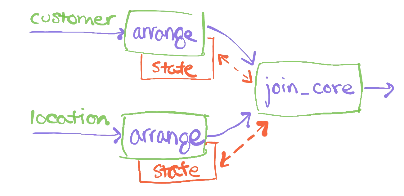
We have broken the traditional join operator into three parts. Each of the inputs first visits an arrange operator, whose results then go to a join_core operator. The arrange operators are in charge of building and maintaining the indexed representations of their inputs. The join_core operator takes two pre-indexed, maintained collections and applies the join logic to the changes that move through them.
Why break apart the join operator into arrange and join_core?
As you may know from relational databases, a small number of indexes can service a large volume of queries. The same is true in Materialize: we can re-use the indexed representations of collections across many independent joins. By separating the operator into 1. data organization and 2. computation, we can more easily slot in shared, re-used arrangements of data. This can result in a substantial reduction in the amount of memory required, as compared to traditional dataflow systems.
Let's take the example above, using customer and location. The standard dataflow system will build private indexes of customer and location, each indexed by their zip field. The zip field in location may be a primary key, meaning each record has a different value of the field. Joins using primary keys are effectively "look-ups" and are quite common. Each such look-up would be a join using location.zip and would require the same index. We can build the index once, and re-use it across all of the query dataflows that need it.
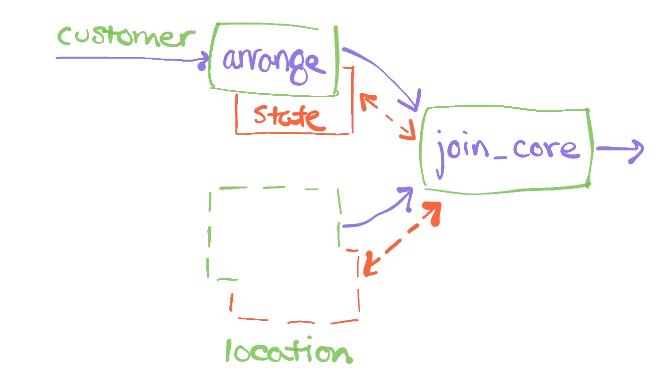
We would still need a private copy of customer indexed by zip, but as we will see next there are standard clever idioms from databases that can make this efficient as well.
Joins in Materialize: TPC-H examples
Let's work through a query from the TPC-H data warehousing benchmark. Query 03 is designed to match the following description:
The Shipping Priority Query retrieves the shipping priority and potential revenue, defined as the sum of l_extendedprice * (1-l_discount), of the orders having the largest revenue among those that had not been shipped as of a given date. Orders are listed in decreasing order of revenue. If more than 10 unshipped orders exist, only the 10 orders with the largest revenue are listed.
The query itself is:
1 | |
2 | |
3 | |
4 | |
5 | |
6 | |
7 | |
8 | |
9 | |
10 | |
11 | |
12 | |
13 | |
14 | |
15 | |
16 | |
17 | |
18 | |
19 | |
20 | |
21 | |
22 | |
The absence of LIMIT 10 from the query is just how TPC-H defines things. In the interest of clarity we are going to work on the core of the query, without the ORDER BY or elided LIMIT. The query is a three-way join between customer, orders, and lineitem, followed by a reduction. The reduction keys seem to be three random fields, but notice that l_orderkey = o_orderkey, where o_orderkey is a primary key for orders; we are producing an aggregate for each order.
We'll be using the scale-factor 1 dataset, as it is what I have locally and it is good enough to call out some of the trade-offs. You can mentally multiply the numbers we'll see by various powers of ten, and the same conclusions will hold.
Joins in Materialize: A first implementation
We can turn on materialize and frame the query above, using the CREATE MATERIALIZED VIEW .. syntax. This instructs materialize to spin up a dataflow to read and maintain the results of the query. We can do this with no other preparation (other than creating the customer, orders, and lineitem data sources).
1 | |
2 | |
3 | |
4 | |
5 | |
6 | |
7 | |
8 | |
9 | |
10 | |
11 | |
12 | |
13 | |
14 | |
15 | |
16 | |
17 | |
18 | |
19 | |
20 | |
At this point, we should have efficient random access to the results. There are many results, so let's just count them instead.
1 | |
2 | |
3 | |
4 | |
5 | |
6 | |
7 | |
8 | |
At the same time, maintaining this query comes with a cost. The dataflow that maintains query_03 maintains several indexes over input and intermediate data. Here is a sketch of what the dataflow graph looks like for the query deployed against the raw data.
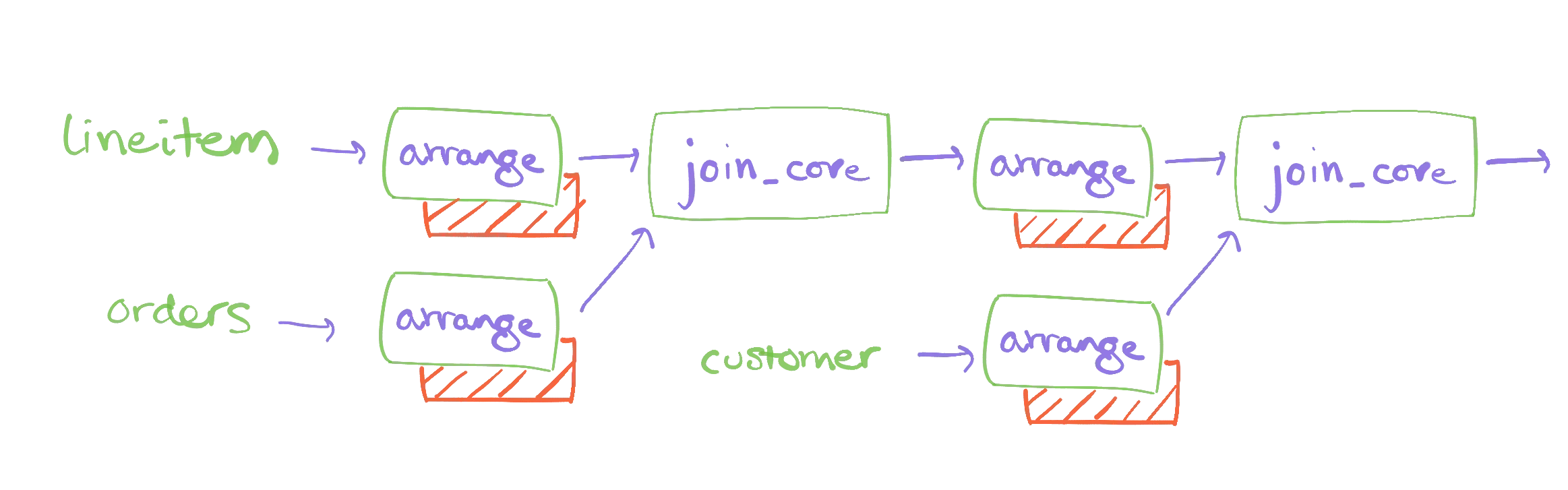
We can read out these volumes from materialize's logging views. To read out the total records maintained by each dataflow, we would type
1 | |
2 | |
3 | |
4 | |
5 | |
When we do, we see (truncated):
1 | |
2 | |
3 | |
4 | |
This tells us that our dataflow maintains some 4,173,794 records for the query_03 dataflow. These are in support of maintaining the 11,620 results from that query, which may seem disproportionate. The explanation is that this dataflow needs to maintain each of its inputs, which are not otherwise stored within materialize. For example, the lineitem relation has six million records, and we need to maintain all relevant records (not all of them, as the filter on date removes roughly half of them).
However, there is a substantial cost to maintaining this query. If we wanted to maintain more queries with similar structure, each would require just as many additional records. We would exhaust the memory of the system relatively quickly as we add these queries.
This approach roughly tracks the resources required by the conventional dataflow processor. So, let's do something smarter.
Joins in Materialize: Primary Indexes
Each of the TPC-H relations have a "primary key": a set of columns such that each record has distinct values for these columns. As discussed above, joins often use primary keys. If we pre-arrange data by its primary key, we might find that we can use those arrangements in the dataflow. This means we may not have to maintain as much per-dataflow state.
Let's build indexes on the primary keys for each collection. We do this with Materialize's CREATE INDEX command.
1 | |
2 | |
3 | |
4 | |
5 | |
6 | |
7 | |
8 | |
These indexes have names, though we do not need to use them explicitly. Rather, the columns identified at the end of each line indicate which columns are used as keys for the index. In this case, they are all primary keys.
We can rebuild our dataflow for query_03 with these indexes in place. Materialize is able to plan the dataflows based on the available indexes, and may find better plans which maintain less private state. The new dataflow graph will looks like so
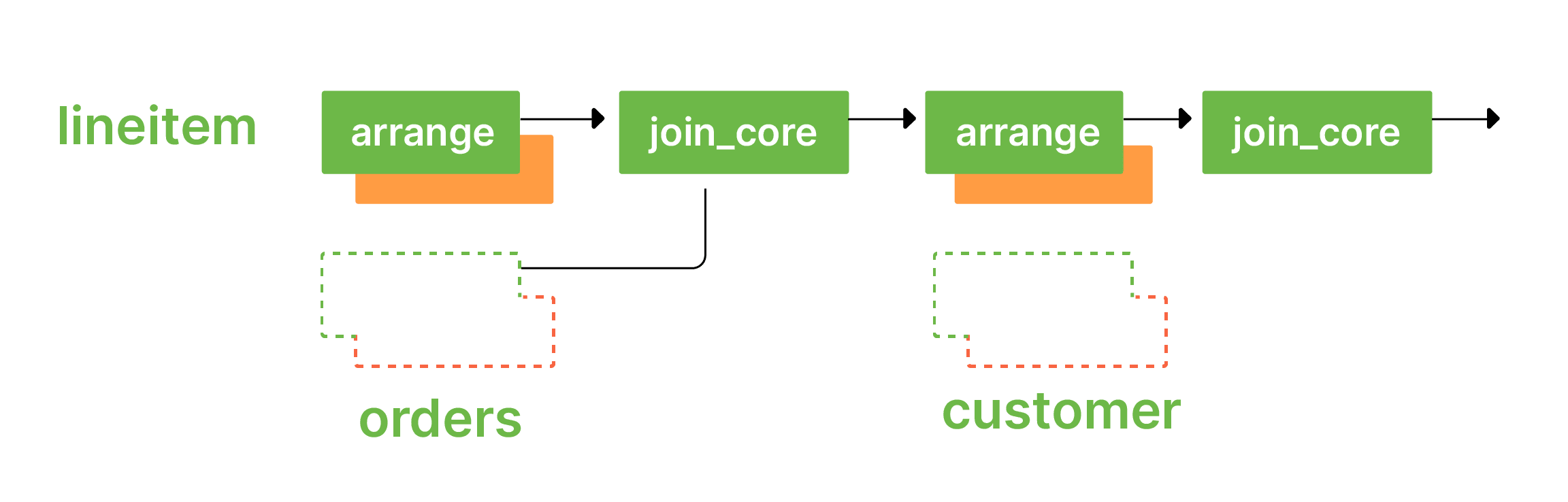
Notice that some of the places where we had "state" before are now dotted. This indicates that they are not new state; the state is simply re-used from pre-existing arrangements.
If we re-run our diagnostic query, the one that counts the records maintained by dataflow, we see
1 | |
2 | |
3 | |
4 | |
5 | |
6 | |
7 | |
8 | |
9 | |
10 | |
There are a few things to notice here. First, there are a lot more entries. Each of the indexes we constructed are backed by dataflows, and they each maintain as many records as their collection contains. Second, the number of records for query_03 has decreased. It has not vanished, and we will explain what records it still maintains, but it is on its way to maintaining fewer records. Third, the numbers for the other indexes are non-trivial. This has not been a net reduction, if we only needed to maintain query_03. However, the conceit is that for multiple queries, the primary indexes are a fixed cost and the per-dataflow reductions apply to each new query.
How do we explain the reduction for query_03? Why was the reduction as much as it was, and why was it not more substantial? If we examine the query, we can see that the equality constraints are on o_orderkey and c_custkey, which are primary keys for orders and customer respectively. However, we do not use (l_orderkey, l_linenumber) which is the primary key for lineitem. This means while we can re-use pre-arranged data for orders and customer, we cannot re-use the pre-arranged data for lineitem. That relation happens to be the large one, and so we still eat the cost of maintaining much of that relation (again, with a filter applied to it).
Joins in Materialize: Secondary Indexes
If we had an arrangement of lineitem by l_orderkey, we should be able to use it, and further reduce the memory requirements. Let's try that now.
1 | |
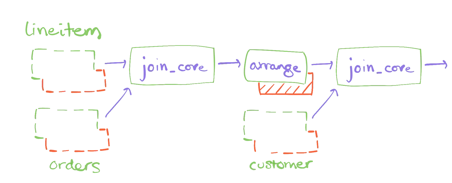
Rebuilding the query results in a dataflow that looks like so
If we re-pull the statistics on records maintained, we see
1 | |
2 | |
3 | |
4 | |
5 | |
6 | |
7 | |
8 | |
9 | |
10 | |
11 | |
The query_03 dataflow is now substantially smaller. We've been able to re-use the fk_lineitem_orderkey arrangement of data, saving ourselves a substantial number of records. This comes at the cost of a new fixed-cost arrangement of data. This is expensive because the index we have described arranges all of lineitem. Readers familiar with databases may wonder why we didn't just create an index from l_orderkey to lineitem's primary key. We'll get to that in a few sections!
Recall from up above that query_03 just has 11,620 records. Where are the remaining 162,951 records coming from?
While we may be able to use pre-arranged inputs for orders, customer, and now lineitem, our dataflow still need to mainain the intermediate results produced from the first binary join. As it turns out this is the result of joining orders and customer, then filtering by the BUILDING constraint. This could be big or small, and fortunately in this case it is not exceedingly large.
However, maintaining these intermediate results gets increasingly painful with multi-way joins that involve more relations. TPC-H query 08 contains an eight-way join, and would have seven intermediate results to maintain. There is no reason to believe that these intermediate results would be substantially smaller than the inputs. Moreover, the intermediate results are almost certainly specific to the query; we wouldn't expect they could be re-used across queries.
Fortunately, there is a neat trick to get around the pesky intermediate results.
Joins in Materialize: Delta Queries
Let's go a bit crazy and create all of the secondary indexes we might want. For each column that is a primary key of another collection, what is called a foreign key, we'll build an index using that column. Repeating the fk_lineitem_orderkey from above, these would be:
1 | |
2 | |
3 | |
4 | |
5 | |
6 | |
7 | |
8 | |
9 | |
10 | |
That's a bunch of indexes. It absolutely represents a significant increase in the fixed costs for working with this dataset. But, let's see what happens when we re-build query_03, and re-pull its record counts.
1 | |
2 | |
3 | |
4 | |
5 | |
6 | |
7 | |
8 | |
9 | |
10 | |
11 | |
12 | |
13 | |
14 | |
15 | |
16 | |
17 | |
18 | |
19 | |
As you can see, we have a whole lot of other indexes in there with large record counts. You can also see (look for the -->) that the record count for query_03 dropped significantly. It is now exactly twice 11,620 which is the number of output records. It turns out this is the bare minimum materialize can make it, based on how we maintain aggregations.
So, despite all that worry about intermediate results, with enough indexes we are somehow able to avoid the cost at all. What happened?
Materialize has access to a join execution strategy we call DeltaQuery that aggressively re-uses arrangements and maintains zero intermediate results. This plan uses a quadratic number of arrangements, with respect to the number of input arrangements. This would be terrible for a conventional dataflow system that cannot share arranged data. For Materialize, as long as there are few enough distinct arrangements, the cost can be much lower. Materialize considers this plan only if all the necessary arrangement already exist, in which case the additional cost of the join is zero.
The dataflow for this plan may be mysterious (the lookup operator goes unexplained for today) but you can see that all arrangements are now dotted:
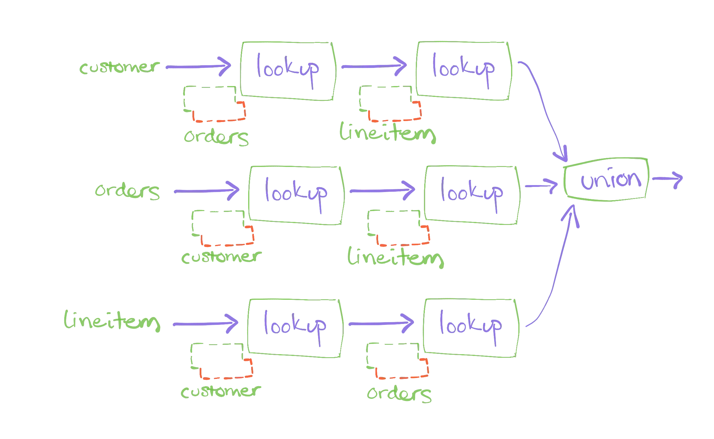
You might reasonably be hesitant about the outlay of pre-arranged data required to enable delta queries. We now have five copies of lineitem to maintain, and it is not the smallest collection of data. However, the per-query cost is now substantially reduced, and a quite-large number of analysts can each work with a quite large number of queries without exhausting materialize.
Joins in Materialize: Late Materialization
For some recently landing bonus content, let's talk about how expensive the five arrangements of lineitem are.
Each of these arrangements replicates the full contents of lineitem. That is clearly a lot of data, and a lot of redundancy. In a conventional dataflow system this overhead is expected; the join operator needs to keep whatever state it needs. But what happens in a more traditional relational database?
Indexes in a relational database don't often replicate the entire collection of data. Rather, they often maintain just a mapping from the indexed columns back to a primary key. These few columns can take substantially less space than the whole collection, and may also change less as various unrelated attributes are updated.
Can we do the same thing in Materialize? Yes!
If we are brave enough to rewrite our query just a little bit, we can write the same join in a way that does not require multiple arrangements of lineitem. The trick will be to define and use a few views that pair foreign and primary keys, and build multiple indexes only on them.
In our case, we only use foreign keys from orders and lineitem, and so we'll just build those views and indexes. More generally, you would build one of these triplets for each foreign key in a collection, mapping it back to a primary key.
1 | |
2 | |
3 | |
4 | |
5 | |
6 | |
7 | |
8 | |
With these new "narrow" views, we can rewrite query_03 to use the narrow views to perform the core equijoin logic. We then join their primary keys back to the orders and lineitem collections, indexed only by their primary keys.
1 | |
2 | |
3 | |
4 | |
5 | |
6 | |
7 | |
8 | |
9 | |
10 | |
11 | |
12 | |
13 | |
14 | |
15 | |
16 | |
17 | |
18 | |
19 | |
20 | |
21 | |
22 | |
23 | |
24 | |
25 | |
26 | |
27 | |
28 | |
What happens now in join planning is that "delta query" planning still kicks in. We have all of the necessary arrangements at hand to avoid maintaining intermediate state. The difference is that we only ever use one arrangement for each of the "wide" relations. The relations that must be multiply arranged are narrow relations whose rows can be substantially smaller.
We've still got some work to do on this pattern, in particular automating it so that you needn't rewrite your query. However, I hope it has hinted at the ways in which Materialize can adapt efficient idioms from traditional databases to the data-parallel streaming setting.
Conclusions
Scanning across the 22 TPC-H queries, the numbers of records each query needs to maintain drops dramatically as we introduce indexes:
*: Query 20 has a doubly nested correlated subquery, and we currently decorrelated this less well than we could. The query does complete after 11 minutes or so, but it runs much more efficiently once manually decorrelated. Query 18 would also be much better manually decorrelated, but it ran to completion so I recorded the numbers.
Joins are a pretty interesting beast in Materialize.
Our use of shared arrangements means gives us access to efficient join plans that conventional dataflow systems cannot support. These join plans can substantially reduce the per-query resource requirements for relational queries.
If you have an interesting collection of relational data which needs joining, check out Materialize now!