How to monitor freshness in Materialize

Freshness measures the time from when a change occurs in an upstream system to when it becomes visible in the results of a query. This guide shows how to track freshness for an object over time and how to summarize a whole window of freshness observations with a CCDF or an HDR histogram.

If freshness is worse than expected, see Freshness troubleshooting to diagnose and resolve the cause.

Track freshness over time

To track freshness for a specific object over time, query its wallclock lag history. The following query returns the last 6 hours of wallclock lag for a materialized view (replace <your_mv_name> with the name of your object):

SELECT wl.occurred_at, wl.lag
FROM mz_internal.mz_wallclock_global_lag_recent_history wl
JOIN mz_catalog.mz_objects o ON wl.object_id = o.id
WHERE o.name = '<your_mv_name>'
  AND wl.occurred_at > now() - INTERVAL '6 hours'
ORDER BY wl.occurred_at DESC;

For example, for a materialized view named freshness_demo, the query returns output like the following:

      occurred_at       |   lag
------------------------+----------
 2026-07-30 19:38:00+00 | 00:00:02
 2026-07-30 19:37:00+00 | 00:00:02
 2026-07-30 19:36:00+00 | 00:00:02
 2026-07-30 19:35:00+00 | 00:00:02
 2026-07-30 19:34:00+00 | 00:00:02
(5 rows)

Each row is one minute-binned observation of the object’s wallclock lag, most recent first. Here lag holds steady at about two seconds, which is the expected, healthy pattern for a lightly loaded object.

Summarize freshness with a CCDF

A raw time series is hard to summarize. A complementary cumulative distribution function (CCDF) compresses a whole window of freshness observations into a compact summary that answers one question: for a given threshold X, what fraction of the time was the object’s freshness at or above X?

This is the compact way to describe a freshness distribution. Instead of staring at a time series, you can make statements like “freshness stayed under 10 seconds 99.9% of the time”. Reading it the other way round, from a percentile to a freshness, needs the HDR histogram below.

The following query builds a freshness CCDF across every object from the last 24 hours of history. It reads the fast, indexed mz_internal.mz_wallclock_global_lag_recent_history and, for a fixed set of decade thresholds (1, 10, and 100 seconds), reports the fraction of observations whose freshness was at or above each threshold. The fixed thresholds mean every run returns all three rows, even when the larger thresholds have no observations:

WITH lags AS (
    -- Convert each lag to seconds, dropping unhydrated (NULL) observations and
    -- any non-positive lag.
    SELECT extract(epoch FROM wl.lag) AS lag_seconds
    FROM mz_internal.mz_wallclock_global_lag_recent_history wl
    WHERE wl.lag IS NOT NULL
      AND wl.lag > INTERVAL '0'
),
thresholds AS (
    -- Fixed decade thresholds, so the CCDF always reports 1s, 10s, and 100s.
    SELECT unnest(ARRAY[1, 10, 100]) AS lag_threshold_seconds
)
SELECT
    t.lag_threshold_seconds,
    count(*) FILTER (WHERE l.lag_seconds >= t.lag_threshold_seconds)::float8
        / count(*) AS fraction_of_time_at_or_above
FROM thresholds t, lags l
GROUP BY t.lag_threshold_seconds
ORDER BY t.lag_threshold_seconds;

The query returns output like the following:

 lag_threshold_seconds | fraction_of_time_at_or_above
-----------------------+------------------------------
                     1 |                            1
                    10 |                            0
                   100 |                            0
(3 rows)

Read this as: freshness was at or above 1 second 100% of the time and never reached 10 seconds or 100 seconds (0% at or above each). This is the healthy pattern for a lightly loaded instance whose objects all sit at a low, near-constant lag, so the 10-second and 100-second thresholds are zero here. A busier instance under real load might show non-zero fractions at those higher thresholds.

By default this query aggregates across every object. To scope the CCDF to a single object, join mz_catalog.mz_objects in the lags CTE and filter on the object name (replace <your_mv_name> with the name of your object):

WITH lags AS (
    -- Convert each lag to seconds, dropping unhydrated (NULL) observations and
    -- any non-positive lag.
    SELECT extract(epoch FROM wl.lag) AS lag_seconds
    FROM mz_internal.mz_wallclock_global_lag_recent_history wl
    JOIN mz_catalog.mz_objects o ON wl.object_id = o.id
    WHERE o.name = '<your_mv_name>'
      AND wl.lag IS NOT NULL
      AND wl.lag > INTERVAL '0'
),
thresholds AS (
    -- Fixed decade thresholds, so the CCDF always reports 1s, 10s, and 100s.
    SELECT unnest(ARRAY[1, 10, 100]) AS lag_threshold_seconds
)
SELECT
    t.lag_threshold_seconds,
    count(*) FILTER (WHERE l.lag_seconds >= t.lag_threshold_seconds)::float8
        / count(*) AS fraction_of_time_at_or_above
FROM thresholds t, lags l
GROUP BY t.lag_threshold_seconds
ORDER BY t.lag_threshold_seconds;

To compare against an SLO, pick your target freshness (say 10 seconds) and read the fraction of time at or above it. That fraction is how often the object was violating the SLO over the window.

Expect a few artifacts in the data. NULL lag rows are unhydrated observations, and the query above already filters them out. If a spurious shelf appears far out at roughly 1.76e9 seconds (about 56 years), it comes from unhydrated collections reported at the Unix epoch, so filter it out (for example with AND wl.lag < INTERVAL '1 year') so it does not distort the fractions.

Summarize freshness with an HDR histogram

A CCDF answers a question you pose in one direction: you pick a threshold, and it tells you what fraction of the time freshness was at or above it. Sometimes you want the other direction. You pick a percentile, and it tells you the freshness. Answering that requires a distribution over many buckets rather than a handful of fixed thresholds.

A High Dynamic Range (HDR) histogram provides one. It buckets observations so that bucket width grows with magnitude: narrow buckets near zero, wide buckets far out. This bounds the relative error of every bucket while keeping the total number of buckets small, which suits lag measurements, where a one-second difference matters at 2s and is noise at 200s. For background on the technique and on exact histograms as an alternative, see Percentile calculation.

The following query buckets the last 24 hours of lag observations and turns the bucket counts into a cumulative distribution. Each lag is converted to seconds and decomposed into significand * 2^exponent. The significand is rounded down to a multiple of 1/16 (4 bits of precision), and the value reconstructed to give the bucket. The final SELECT divides each bucket’s cumulative count by the total count:

WITH
  lags AS (
      -- Convert each lag to seconds, dropping unhydrated (NULL) observations,
      -- any non-positive lag, and the epoch shelf described in the CCDF
      -- section above.
      SELECT extract(epoch FROM wl.lag) AS lag_seconds
      FROM mz_internal.mz_wallclock_global_lag_recent_history wl
      WHERE wl.lag IS NOT NULL
        AND wl.lag > INTERVAL '0'
        AND wl.lag < INTERVAL '1 year'
  ),
  lag_exponents AS (
      -- Decompose each lag into significand * 2^exponent.
      SELECT lag_seconds, floor(log(2, lag_seconds))::int AS exponent
      FROM lags
  ),
  buckets AS (
      -- Reduce the significand by 4 bits, rounding the value down to the
      -- nearest multiple of 1/16, then reconstruct it to get the bucket.
      SELECT
          trunc(lag_seconds / pow(2.0, exponent) * pow(2.0, 4)) / pow(2.0, 4)
              * pow(2.0, exponent) AS bucket_seconds
      FROM lag_exponents
  ),
  histogram AS (
      SELECT bucket_seconds, count(*) AS count_of_bucket_values
      FROM buckets
      GROUP BY bucket_seconds
  )
SELECT
    h.bucket_seconds,
    h.count_of_bucket_values,
    sum(g.count_of_bucket_values) AS cumulative_count,
    sum(g.count_of_bucket_values)::float8
        / (SELECT sum(count_of_bucket_values) FROM histogram)
        AS cumulative_density
FROM histogram g, histogram h
WHERE g.bucket_seconds <= h.bucket_seconds
GROUP BY h.bucket_seconds, h.count_of_bucket_values
ORDER BY h.bucket_seconds;

The query returns output like the following:

 bucket_seconds | count_of_bucket_values | cumulative_count | cumulative_density
----------------+------------------------+------------------+--------------------
              1 |                   7613 |             7613 | 0.9450099304865939
              2 |                    366 |             7979 |  0.990441906653426
              3 |                     32 |             8011 | 0.9944141012909633
              4 |                     36 |             8047 | 0.9988828202581926
              5 |                      7 |             8054 | 0.9997517378351539
              6 |                      2 |             8056 |                  1
(6 rows)

Every bucket here is a whole number of seconds, because at this range 4 bits of significand precision is finer than the 1s resolution of the measurement itself. The buckets only start to widen further out, and 4 bits hold every one of them to within about 6% of the values it contains, so the bucket count stays bounded however far the tail runs.

To read a percentile, take the lowest bucket whose cumulative density reaches it. Wrapping the distribution in one more CTE and filtering on cumulative_density returns the approximate p99 freshness:

WITH
  lags AS (
      SELECT extract(epoch FROM wl.lag) AS lag_seconds
      FROM mz_internal.mz_wallclock_global_lag_recent_history wl
      WHERE wl.lag IS NOT NULL
        AND wl.lag > INTERVAL '0'
        AND wl.lag < INTERVAL '1 year'
  ),
  lag_exponents AS (
      SELECT lag_seconds, floor(log(2, lag_seconds))::int AS exponent
      FROM lags
  ),
  buckets AS (
      SELECT
          trunc(lag_seconds / pow(2.0, exponent) * pow(2.0, 4)) / pow(2.0, 4)
              * pow(2.0, exponent) AS bucket_seconds
      FROM lag_exponents
  ),
  histogram AS (
      SELECT bucket_seconds, count(*) AS count_of_bucket_values
      FROM buckets
      GROUP BY bucket_seconds
  ),
  distribution AS (
      SELECT
          h.bucket_seconds,
          sum(g.count_of_bucket_values)::float8
              / (SELECT sum(count_of_bucket_values) FROM histogram)
              AS cumulative_density
      FROM histogram g, histogram h
      WHERE g.bucket_seconds <= h.bucket_seconds
      GROUP BY h.bucket_seconds
  )
SELECT bucket_seconds AS approximate_p99
FROM distribution
WHERE cumulative_density >= 0.99
ORDER BY cumulative_density
LIMIT 1;

 approximate_p99
-----------------
               2
(1 row)

The bucket is a lower bound: the true p99 lies between this bucket and the next one up. Raising the significand precision from 4 bits narrows that interval at the cost of more buckets; lowering it does the reverse.

By default these queries aggregate across every object. To scope them to a single object, join mz_catalog.mz_objects in the lags CTE and filter on the object name, as in the CCDF section above.

Reading percentiles off a table works, but a percentile plot shows the whole distribution at once. Lag goes on a log vertical axis, and the percentile on a log-probability horizontal axis, so each additional nine gets the same width. A linear percentile axis would crush every nine past the first into the last few pixels, which is exactly where the interesting behaviour lives:

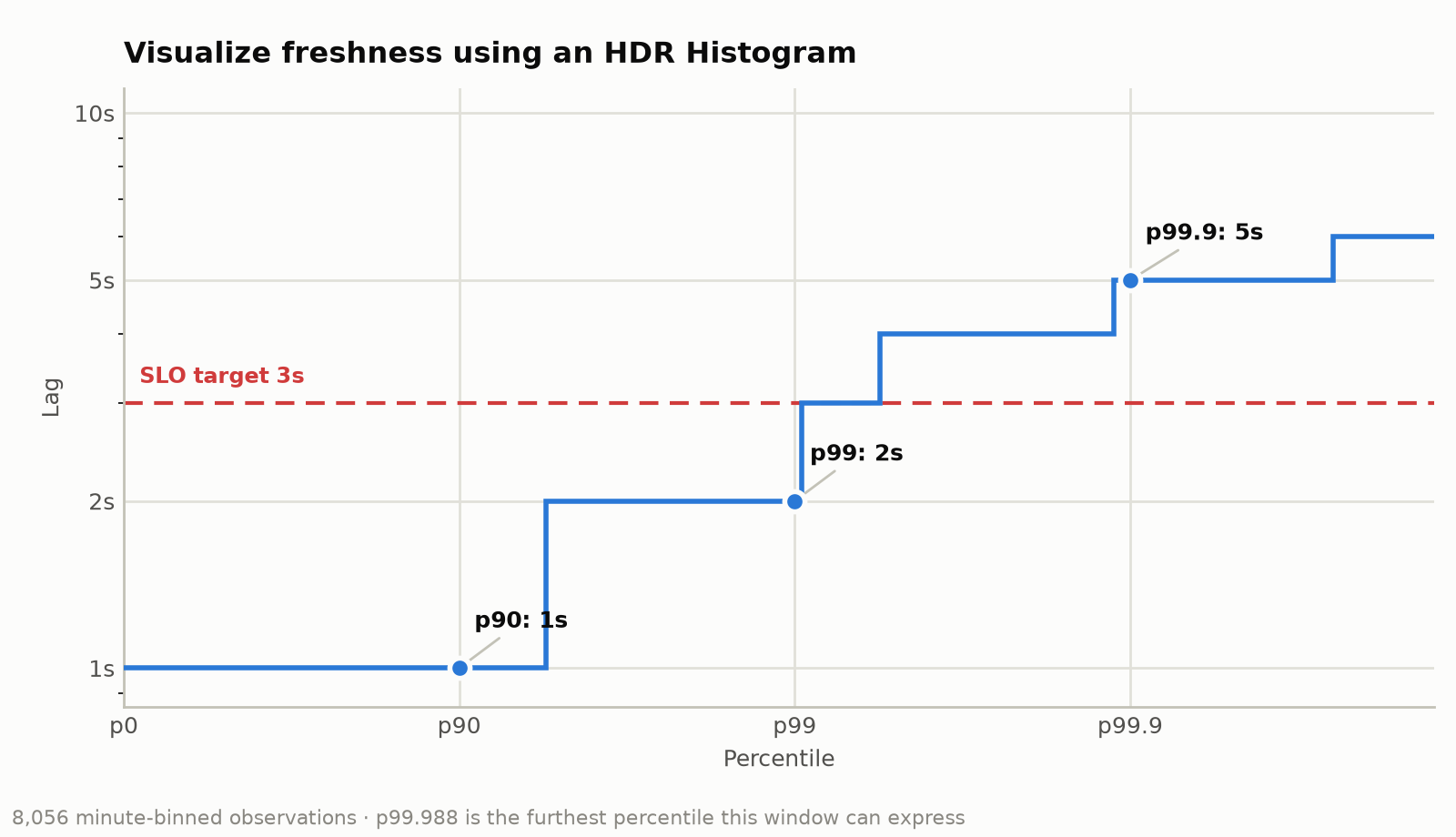
Read it by picking a percentile along the bottom and reading the lag off the left, which is the lookup the p99 query above performs. Each step up is one bucket boundary. Where the curve crosses the SLO line is the percentile at which the target stops holding, so a curve that crosses early is failing the target more often than one that crosses late.

The curve has to stop somewhere: a window of N observations cannot express a percentile beyond 1 - 1/N, because past that there is less than one observation left to place. That is why the right-hand end is annotated with the furthest percentile the window supports rather than running to p100.